Mean Absolute Error (MAE) Loss Function - Derivatives and Gradients (导数和梯度)

Mean Absolute Error {MAE} Loss Function - Derivatives and Gradients {导数和梯度}

• [1. torch.nn.L1Loss](#1. torch.nn.L1Loss)
• • [1.1. Parameters](#1.1. Parameters)
  • [1.2. Shape](#1.2. Shape)
  • [1.3. `torch.nn.L1Loss(size_average=None, reduce=None, reduction='mean')`](#1.3. torch.nn.L1Loss(size_average=None, reduce=None, reduction='mean'))
  • [1.4. `torch.nn.L1Loss(size_average=None, reduce=None, reduction='sum')`](#1.4. torch.nn.L1Loss(size_average=None, reduce=None, reduction='sum'))
• [2. sign function or signum function](#2. sign function or signum function)
• • [2.1. Basic properties](#2.1. Basic properties)
  • [2.2. numpy.sign](#2.2. numpy.sign)
• [3. Mean Absolute Error (MAE) Loss Function - Derivatives and Gradients (导数和梯度)](#3. Mean Absolute Error (MAE) Loss Function - Derivatives and Gradients (导数和梯度))
• [4. Mean Absolute Error (MAE) Loss Function - Derivatives and Gradients (导数和梯度)](#4. Mean Absolute Error (MAE) Loss Function - Derivatives and Gradients (导数和梯度))
• • [4.1. PyTorch `torch.nn.L1Loss(size_average=None, reduce=None, reduction='mean')`](#4.1. PyTorch torch.nn.L1Loss(size_average=None, reduce=None, reduction='mean'))
  • [4.2. PyTorch `torch.nn.L1Loss(size_average=None, reduce=None, reduction='mean')`](#4.2. PyTorch torch.nn.L1Loss(size_average=None, reduce=None, reduction='mean'))
  • [4.3. Python `torch.nn.L1Loss(size_average=None, reduce=None, reduction='mean')`](#4.3. Python torch.nn.L1Loss(size_average=None, reduce=None, reduction='mean'))
  • [4.4. Python `torch.nn.L1Loss(size_average=None, reduce=None, reduction='mean')`](#4.4. Python torch.nn.L1Loss(size_average=None, reduce=None, reduction='mean'))
• References

1. torch.nn.L1Loss

https://docs.pytorch.org/docs/stable/generated/torch.nn.L1Loss.html
https://github.com/pytorch/pytorch/blob/main/torch/nn/modules/loss.py

class torch.nn.L1Loss(size_average=None, reduce=None, reduction='mean')

Creates a criterion that measures the mean absolute error (MAE) between each element in the input x x x and target y y y.

The unreduced (i.e. with reduction set to 'none') loss can be described as:

ℓ ( x , y ) = L = { l 1 , ... , l N } ⊤ , l n = ∣ x n − y n ∣ , \ell(x, y) = L = \{l_1,\dots,l_N\}^\top, \quad l_n = \left| x_n - y_n \right|, ℓ(x,y)=L={l1,...,lN}⊤,ln=∣xn−yn∣,

where N N N is the batch size.

If reduction is not 'none' (default 'mean'), then:

ℓ ( x , y ) = { mean ⁡ ( L ) , if reduction = 'mean'; sum ⁡ ( L ) , if reduction = 'sum'. \ell(x, y) = \begin{cases} \operatorname{mean}(L), & \text{if reduction} = \text{'mean';}\\ \operatorname{sum}(L), & \text{if reduction} = \text{'sum'.} \end{cases} ℓ(x,y)={mean(L),sum(L),if reduction='mean';if reduction='sum'.

x x x and y y y are tensors of arbitrary shapes with a total of N N N elements each.

The sum operation still operates over all the elements, and divides by N N N.

The division by N N N can be avoided if one sets reduction = 'sum'.

Supports real-valued and complex-valued inputs.

1.1. Parameters

• size_average (bool, optional): Deprecated (see reduction). By default, the losses are averaged over each loss element in the batch. Note that for some losses, there are multiple elements per sample. If the field size_average is set to False, the losses are instead summed for each minibatch. Ignored when reduce is False. Default: True

• reduce (bool, optional): Deprecated (see reduction). By default, the losses are averaged or summed over observations for each minibatch depending on size_average. When reduce is False, returns a loss per batch element instead and ignores size_average. Default: True

• reduction (str, optional): Specifies the reduction to apply to the output: 'none' | 'mean' | 'sum'. 'none': no reduction will be applied, 'mean': the sum of the output will be divided by the number of elements in the output, 'sum': the output will be summed. Note: size_average and reduce are in the process of being deprecated, and in the meantime, specifying either of those two args will override reduction. Default: 'mean'

1.2. Shape

• Input : (*), where * means any number of dimensions.

• Target : (*), same shape as the input.

• Output : scalar. If reduction is 'none', then (*), same shape as the input.

1.3. torch.nn.L1Loss(size_average=None, reduce=None, reduction='mean')

y_true: Ground truth values with shape = [d1, d2, ..., dN].
y_pred: The predicted values with shape = [d1, d2, ..., dN]. (Tensor of the same shape as y_true)

MAELoss (mean) = np.mean(np.abs(y_pred - y_true))

Mean Absolute Error (MAE):

MAE (mean) = 1 d 1 × d 2 × . . . × d N ∑ i = 1 d 1 × d 2 × . . . × d N ∣ y _ p r e d i − y _ t r u e i ∣ \begin{aligned} \text{MAE (mean)} &= \frac{1}{d1 \times d2 \times ... \times dN} \sum_{i=1}^{d1 \times d2 \times ... \times dN} |\boldsymbol{y\pred}{i} - \boldsymbol{y\true}{i}| \\ \end{aligned} MAE (mean)=d1×d2×...×dN1i=1∑d1×d2×...×dN∣y_predi−y_truei∣

The MAE function gradient (Tensor of the same shape as y_pred):

J ( mean ) = ∂ L ∂ y ^ = 1 d 1 × d 2 × . . . × d N sgn ( y _ p r e d − y _ t r u e ) \begin{aligned} \boldsymbol{J (\text{mean})} &= \frac{\partial{L}}{\partial{\boldsymbol{\hat{y}}}} \\ &= \frac{1}{d1 \times d2 \times ... \times dN} \text{sgn}(\boldsymbol{y\_pred} - \boldsymbol{y\_true}) \\ \end{aligned} J(mean)=∂y^∂L=d1×d2×...×dN1sgn(y_pred−y_true)

1.4. torch.nn.L1Loss(size_average=None, reduce=None, reduction='sum')

y_true: Ground truth values with shape = [d1, d2, ..., dN].
y_pred: The predicted values with shape = [d1, d2, ..., dN]. (Tensor of the same shape as y_true)

MAELoss (sum) = np.sum(np.abs(y_pred - y_true))

Mean Absolute Error (MAE):

MAE (sum) = ∑ i = 1 d 1 × d 2 × . . . × d N ∣ y _ p r e d i − y _ t r u e i ∣ \begin{aligned} \text{MAE (sum)} &= \sum_{i=1}^{d1 \times d2 \times ... \times dN} |\boldsymbol{y\pred}{i} - \boldsymbol{y\true}{i}| \\ \end{aligned} MAE (sum)=i=1∑d1×d2×...×dN∣y_predi−y_truei∣

The MAE function gradient (Tensor of the same shape as y_pred):

J ( sum ) = ∂ L ∂ y ^ = sgn ( y _ p r e d − y _ t r u e ) \begin{aligned} \boldsymbol{J (\text{sum})} &= \frac{\partial{L}}{\partial{\boldsymbol{\hat{y}}}} \\ &= \text{sgn} (\boldsymbol{y\_pred} - \boldsymbol{y\_true}) \\ \end{aligned} J(sum)=∂y^∂L=sgn(y_pred−y_true)

2. sign function or signum function

In mathematics, the sign function or signum function is a function that has the value -1, +1 or 0 according to whether the sign of a given real number is positive or negative, or the given number is itself zero.

In mathematical notation the sign function is often represented as sgn x \text{sgn} \ x sgn x or sgn ( x ) \text{sgn} (x) sgn(x).

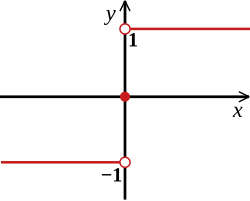
sgn ( x ) = { − 1 if x < 0 0 if x = 0 1 if x > 0 \text{sgn} (x) = \begin{cases} -1 & \text{if} \ x < 0 \\ 0 & \text{if} \ x = 0 \\ 1 & \text{if} \ x > 0 \\ \end{cases} sgn(x)=⎩ ⎨ ⎧−101if x<0if x=0if x>0

For example:

sgn ( 2 ) = + 1 sgn ( π ) = + 1 sgn ( − 8 ) = − 1 sgn ( − 1 2 ) = − 1 sgn ( 0 ) = 0 \begin{aligned} \text{sgn}(2) &=& +1 \\ \text{sgn}(\pi) &=& +1 \\ \text{sgn}(-8) &=& -1 \\ \text{sgn}(-\frac{1}{2}) &=& -1 \\ \text{sgn}(0) &=& 0 \\ \end{aligned} sgn(2)sgn(π)sgn(−8)sgn(−21)sgn(0)=====+1+1−1−10

2.1. Basic properties

Any real number can be expressed as the product of its absolute value and its sign:
x = ∣ x ∣ sgn x x = |x| \text{sgn} x x=∣x∣sgnx

It follows that whenever x {x} x is not equal to 0 we have
sgn x = x ∣ x ∣ = ∣ x ∣ x \text{sgn} x = \frac{x}{|x|} = \frac{|x|}{x} sgnx=∣x∣x=x∣x∣

Similarly, for any real number x x x,
∣ x ∣ = x sgn x |x| = x \text{sgn} x ∣x∣=xsgnx

2.2. numpy.sign

https://numpy.org/doc/stable/reference/generated/numpy.sign.html

Returns an element-wise indication of the sign of a number.

The sign function returns -1 if x < 0, 0 if x==0, 1 if x > 0. nan is returned for nan inputs.

Notes

There is more than one definition of sign in common use for complex numbers. The definition used here, x / ∣ x ∣ x/|x| x/∣x∣, is the more common and useful one, but is different from the one used in numpy prior to version 2.0, x / x × x x/\sqrt{x \times x} x/x×x , which is equivalent to sign(x.real) + 0j if x.real != 0 else sign(x.imag) + 0j.

3. Mean Absolute Error (MAE) Loss Function - Derivatives and Gradients (导数和梯度)

Predicted values:

y _ p r e d = y ^ = [ y ^ 1 , y ^ 2 , ... , y ^ N ] \boldsymbol{y\pred} = \boldsymbol{\hat{y}} = \left[ \hat{y}{1}, \hat{y}{2}, \dots, \hat{y}{N} \right ] y_pred=y^=[y^1,y^2,...,y^N]

True values:

y _ t r u e = y = [ y 1 , y 2 , ... , y N ] \boldsymbol{y\true} = \boldsymbol{y} = \left[ {y}{1}, {y}{2}, \dots, {y}{N} \right ] y_true=y=[y1,y2,...,yN]

Mean Absolute Error (MAE):

MAE = L = 1 N ∑ i = 1 N ∣ y _ p r e d i − y _ t r u e i ∣ = 1 N ∑ i = 1 N ∣ y ^ i − y i ∣ = 1 N ( ∣ y ^ 1 − y 1 ∣ + ∣ y ^ 2 − y 2 ∣ + ... + ∣ y ^ N − y N ∣ ) \begin{aligned} \text{MAE} = L &= \frac{1}{N} \sum_{i=1}^{N}|\boldsymbol{y\pred}{i} - \boldsymbol{y\true}{i}| \\ &= \frac{1}{N} \sum_{i=1}^{N} |\boldsymbol{\hat{y}}{i} - \boldsymbol{y}{i}| \\ &= \frac{1}{N} (|\hat{y}{1} - {y}{1}| + |\hat{y}{2} - {y}{2}| + \ldots + |\hat{y}{N} - {y}{N}|) \\ \end{aligned} MAE=L=N1i=1∑N∣y_predi−y_truei∣=N1i=1∑N∣y^i−yi∣=N1(∣y^1−y1∣+∣y^2−y2∣+...+∣y^N−yN∣)

其中 MAE = L \text{MAE} = L MAE=L 是标量， N N N 是常量。

The partial derivative with respect to y ^ j \hat{y}_{j} y^j is:

∂ L ∂ y ^ j = ∂ ∂ y ^ j 1 N ∑ i = 1 N ∣ y ^ i − y i ∣ = 1 N ∂ ∂ y ^ j ∑ i = 1 N ∣ y ^ i − y i ∣ = 1 N ∑ i = 1 N ∂ ∂ y ^ j ∣ y ^ i − y i ∣ \begin{aligned} \frac{\partial{L}}{\partial{\hat{y}{j}}} &= \frac{\partial{}}{\partial{\hat{y}{j}}} \frac{1}{N} \sum_{i=1}^{N} |\boldsymbol{\hat{y}}{i} - \boldsymbol{y}{i}| \\ &= \frac{1}{N} \frac{\partial{}}{\partial{\hat{y}{j}}} \sum{i=1}^{N} |\boldsymbol{\hat{y}}{i} - \boldsymbol{y}{i}| \\ &= \frac{1}{N} \sum_{i=1}^{N} \frac{\partial{}}{\partial{\hat{y}{j}}} |\boldsymbol{\hat{y}}{i} - \boldsymbol{y}_{i}| \\ \end{aligned} ∂y^j∂L=∂y^j∂N1i=1∑N∣y^i−yi∣=N1∂y^j∂i=1∑N∣y^i−yi∣=N1i=1∑N∂y^j∂∣y^i−yi∣

If i ≠ j i\neq j i=j, then ∣ y ^ i − y i ∣ |\hat{y}i - y_i| ∣y^i−yi∣ is not a function of y ^ j \hat{y}{j} y^j, so ∂ ∂ y ^ j ∣ y ^ i − y i ∣ = 0 \frac{\partial}{\partial \hat{y}_{j}}|\hat{y}_i - y_i| = 0 ∂y^j∂∣y^i−yi∣=0. We can remove the summation because the partial derivative of L L L for i ≠ j i\neq j i=j is 0. We are left with only one term in the sum, where i = j i=j i=j:

∂ L ∂ y ^ j = ∂ ∂ y ^ j 1 N ∑ i = 1 N ∣ y ^ i − y i ∣ = 1 N ∂ ∂ y ^ j ∑ i = 1 N ∣ y ^ i − y i ∣ = 1 N ∑ i = 1 N ∂ ∂ y ^ j ∣ y ^ i − y i ∣ = 1 N ∂ ∂ y ^ j ∣ y ^ j − y j ∣ = 1 N sgn ( y ^ j − y j ) ∂ ∂ y ^ j ( y ^ j − y j ) = 1 N sgn ( y ^ j − y j ) = 1 N y ^ j − y j ∣ y ^ j − y j ∣ = 1 N ∣ y ^ j − y j ∣ y ^ j − y j \begin{aligned} \frac{\partial{L}}{\partial{\hat{y}{j}}} &= \frac{\partial{}}{\partial{\hat{y}{j}}} \frac{1}{N} \sum_{i=1}^{N} |\boldsymbol{\hat{y}}{i} - \boldsymbol{y}{i}| \\ &= \frac{1}{N} \frac{\partial{}}{\partial{\hat{y}{j}}} \sum{i=1}^{N} |\boldsymbol{\hat{y}}{i} - \boldsymbol{y}{i}| \\ &= \frac{1}{N} \sum_{i=1}^{N} \frac{\partial{}}{\partial{\hat{y}{j}}} |\boldsymbol{\hat{y}}{i} - \boldsymbol{y}{i}| \\ &= \frac{1}{N} \frac{\partial{}}{\partial{\hat{y}{j}}} |\hat{y}{j} - y{j}| \\ &= \frac{1}{N} \text{sgn}(\hat{y}{j} - y{j}) \frac{\partial{}}{\partial{\hat{y}{j}}} (\hat{y}{j} - y_{j}) \\ &= \frac{1}{N} \text{sgn}(\hat{y}{j} - y{j}) \\ &= \frac{1}{N} \frac{\hat{y}{j} - y{j}}{|\hat{y}{j} - y{j}|} \\ &= \frac{1}{N} \frac{|\hat{y}{j} - y{j}|}{\hat{y}{j} - y{j}} \\ \end{aligned} ∂y^j∂L=∂y^j∂N1i=1∑N∣y^i−yi∣=N1∂y^j∂i=1∑N∣y^i−yi∣=N1i=1∑N∂y^j∂∣y^i−yi∣=N1∂y^j∂∣y^j−yj∣=N1sgn(y^j−yj)∂y^j∂(y^j−yj)=N1sgn(y^j−yj)=N1∣y^j−yj∣y^j−yj=N1y^j−yj∣y^j−yj∣

Finally, the gradient ∂ L ∂ y ^ \frac{\partial{L}}{\partial{\hat{\boldsymbol{y}}}} ∂y^∂L is the vector whose j j j-th component is ∂ L ∂ y ^ j \frac{\partial{L}}{\partial{\hat{y}{j}}} ∂y^j∂L, so we have ∂ L ∂ y ^ = 1 N sgn ( y ^ j − y j ) \frac{\partial{L}}{\partial{\hat{\boldsymbol{y}}}} = \frac{1}{N} \text{sgn}(\boldsymbol{\hat{y}}{j} - \boldsymbol{y}_{j}) ∂y^∂L=N1sgn(y^j−yj).

The MAE function gradient (Jacobian for MAE):

MAE = L = f ( y ^ 1 , y ^ 2 , ... , y ^ N ) \begin{aligned} \text{MAE} = L &= f({\hat{y}}{1}, {\hat{y}}{2}, \ \ldots, {\hat{y}}_{N}) \\ \end{aligned} MAE=L=f(y^1,y^2, ...,y^N)

J = ∂ L ∂ y ^ = ∂ L ∂ ( y ^ 1 , y ^ 2 , ... , y ^ N ) = [ ∂ L ∂ y ^ 1 , ∂ L ∂ y ^ 2 , ... , ∂ L ∂ y ^ N ] = [ 1 N sgn ( y ^ 1 − y 1 ) , 1 N sgn ( y ^ 2 − y 2 ) , ... , 1 N sgn ( y ^ N − y N ) ] = 1 N [ sgn ( y ^ 1 − y 1 ) , sgn ( y ^ 2 − y 2 ) , ... , sgn ( y ^ N − y N ) ] = 1 N sgn ( y ^ − y ) = 1 N sgn ( y _ p r e d − y _ t r u e ) = 1 N y ^ − y ∣ y ^ − y ∣ = 1 N ∣ y ^ − y ∣ y ^ − y \begin{aligned} \boldsymbol{J} &= \frac{\partial{L}}{\partial{\boldsymbol{\hat{y}}}} \\ &= \frac{\partial{L}}{\partial{({\hat{y}}{1}, {\hat{y}}{2}, \ \ldots, {\hat{y}}{N})}} \\ &= \left[\frac{\partial{L}}{\partial{\hat{y}{1}}}, \frac{\partial{L}}{\partial{\hat{y}{2}}}, \ \ldots, \frac{\partial{L}}{\partial{\hat{y}{N}}} \right] \\ &= \left[\frac{1}{N} \text{sgn}(\hat{y}{1} - y{1}), \frac{1}{N} \text{sgn}(\hat{y}{2} - y{2}), \ \ldots, \frac{1}{N} \text{sgn}(\hat{y}{N} - y{N}) \right] \\ &= \frac{1}{N} \left[\text{sgn}(\hat{y}{1} - y{1}), \text{sgn}(\hat{y}{2} - y{2}), \ \ldots, \text{sgn}(\hat{y}{N} - y{N}) \right] \\ &= \frac{1}{N} \text{sgn}(\boldsymbol{\hat{y}} - \boldsymbol{y}) \\ &= \frac{1}{N} \text{sgn}(\boldsymbol{y\_pred} - \boldsymbol{y\_true}) \\ &= \frac{1}{N} \frac{\boldsymbol{\hat{y}} - \boldsymbol{y}}{|\boldsymbol{\hat{y}} - \boldsymbol{y}|} \\ &= \frac{1}{N} \frac{|\boldsymbol{\hat{y}} - \boldsymbol{y}|}{\boldsymbol{\hat{y}} - \boldsymbol{y}} \\ \end{aligned} J=∂y^∂L=∂(y^1,y^2, ...,y^N)∂L=[∂y^1∂L,∂y^2∂L, ...,∂y^N∂L]=[N1sgn(y^1−y1),N1sgn(y^2−y2), ...,N1sgn(y^N−yN)]=N1[sgn(y^1−y1),sgn(y^2−y2), ...,sgn(y^N−yN)]=N1sgn(y^−y)=N1sgn(y_pred−y_true)=N1∣y^−y∣y^−y=N1y^−y∣y^−y∣

4. Mean Absolute Error (MAE) Loss Function - Derivatives and Gradients (导数和梯度)

4.1. PyTorch torch.nn.L1Loss(size_average=None, reduce=None, reduction='mean')

#!/usr/bin/env python
# coding=utf-8

import torch
import torch.nn as nn

predictions = torch.tensor([1, 2, 3, 4], dtype=torch.float, requires_grad=True)
targets = torch.tensor([0, 2, 4, 2], dtype=torch.float)

print(f"predictions.requires_grad: {predictions.requires_grad}, targets.requires_grad: {targets.requires_grad}")
print(f"predictions.shape: {predictions.shape}, targets.shape: {targets.shape}")

# Compute MAE loss
mae_loss = nn.L1Loss(size_average=None, reduce=None, reduction='mean')
loss = mae_loss(predictions, targets)
print(f"MAE loss: {loss}")

# Compute gradients
loss.backward()

# Access the gradients of 'predictions'
print(f"\ngradients of predictions:\n{predictions.grad}")
print(f"predictions.shape: {predictions.shape}")

Predicted values:

y _ p r e d = y ^ = [ y ^ 1 , y ^ 2 , ... , y ^ N ] = [ 1 , 2 , 3 , 4 ] \begin{aligned} \boldsymbol{y\pred} = \boldsymbol{\hat{y}} &= \left[ \hat{y}{1}, \hat{y}{2}, \dots, \hat{y}{N} \right] \\ &= \left[ 1, 2, 3, 4 \right] \\ \end{aligned} y_pred=y^=[y^1,y^2,...,y^N]=[1,2,3,4]

True values:

y _ t r u e = y = [ y 1 , y 2 , ... , y N ] = [ 0 , 2 , 4 , 2 ] \begin{aligned} \boldsymbol{y\true} = \boldsymbol{y} &= \left[ {y}{1}, {y}{2}, \dots, {y}{N} \right] \\ &= \left[ 0, 2, 4, 2 \right] \\ \end{aligned} y_true=y=[y1,y2,...,yN]=[0,2,4,2]

Mean Absolute Error (MAE):

MAE = L = 1 N ∑ i = 1 N ∣ y _ p r e d i − y _ t r u e i ∣ = 1 N ∑ i = 1 N ∣ y ^ i − y i ∣ = 1 N ( ∣ y ^ 1 − y 1 ∣ + ∣ y ^ 2 − y 2 ∣ + ... + ∣ y ^ N − y N ∣ ) = 1 4 ( ∣ 1 − 0 ∣ + ∣ 2 − 2 ∣ + ∣ 3 − 4 ∣ + ∣ 4 − 2 ∣ ) = 1.0 \begin{aligned} \text{MAE} = L &= \frac{1}{N} \sum_{i=1}^{N} |\boldsymbol{y\pred}{i} - \boldsymbol{y\true}{i}| \\ &= \frac{1}{N} \sum_{i=1}^{N} |\boldsymbol{\hat{y}}{i} - \boldsymbol{y}{i}| \\ &= \frac{1}{N} (|\hat{y}{1} - {y}{1}| + |\hat{y}{2} - {y}{2}| + \ldots + |\hat{y}{N} - {y}{N}|) \\ &= \frac{1}{4} (|1 - 0| + |2 - 2| + |3 - 4| + |4 - 2|) \\ &= 1.0 \\ \end{aligned} MAE=L=N1i=1∑N∣y_predi−y_truei∣=N1i=1∑N∣y^i−yi∣=N1(∣y^1−y1∣+∣y^2−y2∣+...+∣y^N−yN∣)=41(∣1−0∣+∣2−2∣+∣3−4∣+∣4−2∣)=1.0

The MAE function gradient (Jacobian for MAE):

J = ∂ L ∂ y ^ = ∂ L ∂ ( y ^ 1 , y ^ 2 , ... , y ^ N ) = [ ∂ L ∂ y ^ 1 , ∂ L ∂ y ^ 2 , ... , ∂ L ∂ y ^ N ] = [ 1 N sgn ( y ^ 1 − y 1 ) , 1 N sgn ( y ^ 2 − y 2 ) , ... , 1 N sgn ( y ^ N − y N ) ] = 1 N [ sgn ( y ^ 1 − y 1 ) , sgn ( y ^ 2 − y 2 ) , ... , sgn ( y ^ N − y N ) ] = 1 4 [ sgn ( 1 − 0 ) , sgn ( 2 − 2 ) , sgn ( 3 − 4 ) , sgn ( 4 − 2 ) ] = 1 4 [ 1 , 0 , − 1 , 1 ] = [ 0.25 , 0 , − 0.25 , 0.25 ] \begin{aligned} \boldsymbol{J} &= \frac{\partial{L}}{\partial{\boldsymbol{\hat{y}}}} \\ &= \frac{\partial{L}}{\partial{({\hat{y}}{1}, {\hat{y}}{2}, \ \ldots, {\hat{y}}{N})}} \\ &= \left[\frac{\partial{L}}{\partial{\hat{y}{1}}}, \frac{\partial{L}}{\partial{\hat{y}{2}}}, \ \ldots, \frac{\partial{L}}{\partial{\hat{y}{N}}} \right] \\ &= \left[\frac{1}{N} \text{sgn}(\hat{y}{1} - y{1}), \frac{1}{N} \text{sgn}(\hat{y}{2} - y{2}), \ \ldots, \frac{1}{N} \text{sgn}(\hat{y}{N} - y{N}) \right] \\ &= \frac{1}{N} \left[\text{sgn}(\hat{y}{1} - y{1}), \text{sgn}(\hat{y}{2} - y{2}), \ \ldots, \text{sgn}(\hat{y}{N} - y{N}) \right] \\ &= \frac{1}{4} \left[\text{sgn}(1 - 0), \text{sgn}(2 - 2), \text{sgn}(3 - 4), \text{sgn}(4 - 2) \right] \\ &= \frac{1}{4} \left[1, 0, -1, 1 \right] \\ &= \left[0.25, 0, -0.25, 0.25 \right] \\ \end{aligned} J=∂y^∂L=∂(y^1,y^2, ...,y^N)∂L=[∂y^1∂L,∂y^2∂L, ...,∂y^N∂L]=[N1sgn(y^1−y1),N1sgn(y^2−y2), ...,N1sgn(y^N−yN)]=N1[sgn(y^1−y1),sgn(y^2−y2), ...,sgn(y^N−yN)]=41[sgn(1−0),sgn(2−2),sgn(3−4),sgn(4−2)]=41[1,0,−1,1]=[0.25,0,−0.25,0.25]

/home/yongqiang/miniconda3/bin/python /home/yongqiang/quantitative_analysis/mae.py 
predictions.requires_grad: True, targets.requires_grad: False
predictions.shape: torch.Size([4]), targets.shape: torch.Size([4])
MAE loss: 1.0

gradients of predictions:
tensor([ 0.2500,  0.0000, -0.2500,  0.2500])
predictions.shape: torch.Size([4])

Process finished with exit code 0

4.2. PyTorch torch.nn.L1Loss(size_average=None, reduce=None, reduction='mean')

#!/usr/bin/env python
# coding=utf-8

import torch
import torch.nn as nn

predictions = torch.tensor([[1, 2, 3], [4, 5, 6], [7, 8, 9]], dtype=torch.float, requires_grad=True)
targets = torch.tensor([[2, 2, 2], [6, 5, 4], [9, 9, 9]], dtype=torch.float)

print(f"predictions.requires_grad: {predictions.requires_grad}, targets.requires_grad: {targets.requires_grad}")
print(f"predictions.shape: {predictions.shape}, targets.shape: {targets.shape}")

# Compute MAE loss
mae_loss = nn.L1Loss(size_average=None, reduce=None, reduction='mean')
loss = mae_loss(predictions, targets)
print(f"MAE loss: {loss}")

# Compute gradients
loss.backward()

# Access the gradients of 'predictions'
print(f"\ngradients of predictions:\n{predictions.grad}")
print(f"predictions.shape: {predictions.shape}")

Predicted values:

y _ p r e d = y ^ = [ 1 , 2 , 3 4 , 5 , 6 7 , 8 , 9 ] \begin{aligned} \boldsymbol{y\_pred} &= \boldsymbol{\hat{y}} \\ &= \begin{bmatrix} 1, 2, 3 \\ 4, 5, 6 \\ 7, 8, 9 \\ \end{bmatrix} \end{aligned} y_pred=y^= 1,2,34,5,67,8,9

True values:

y _ t r u e = y = [ 2 , 2 , 2 6 , 5 , 4 9 , 9 , 9 ] \begin{aligned} \boldsymbol{y\_true} &= \boldsymbol{y} \\ &= \begin{bmatrix} 2, 2, 2 \\ 6, 5, 4 \\ 9, 9, 9 \\ \end{bmatrix} \end{aligned} y_true=y= 2,2,26,5,49,9,9

Mean Absolute Error (MAE):

MAE = L = 1 N ∑ i = 1 N ∣ y _ p r e d i − y _ t r u e i ∣ = 1 N ∑ i = 1 N ∣ y ^ i − y i ∣ = 1 3 × 3 ( ∣ 1 − 2 ∣ + ∣ 2 − 2 ∣ + ∣ 3 − 2 ∣ + ∣ 4 − 6 ∣ + ∣ 5 − 5 ∣ + ∣ 6 − 4 ∣ + ∣ 7 − 9 ∣ + ∣ 8 − 9 ∣ + ∣ 9 − 9 ∣ ) = 1 9 × 9 = 1.0 \begin{aligned} \text{MAE} = L &= \frac{1}{N} \sum_{i=1}^{N} |\boldsymbol{y\pred}{i} - \boldsymbol{y\true}{i}| \\ &= \frac{1}{N} \sum_{i=1}^{N} |\boldsymbol{\hat{y}}{i} - \boldsymbol{y}{i}| \\ &= \frac{1}{3 \times 3} (|1 - 2| + |2 - 2| + |3 - 2| + |4 - 6| + |5 - 5| + |6 - 4| + |7 - 9| + |8 - 9| + |9 - 9|) \\ &= \frac{1}{9} \times 9 \\ &= 1.0 \\ \end{aligned} MAE=L=N1i=1∑N∣y_predi−y_truei∣=N1i=1∑N∣y^i−yi∣=3×31(∣1−2∣+∣2−2∣+∣3−2∣+∣4−6∣+∣5−5∣+∣6−4∣+∣7−9∣+∣8−9∣+∣9−9∣)=91×9=1.0

The MAE function gradient (Jacobian for MAE):

J = ∂ L ∂ y ^ = ∂ L ∂ ( y ^ 1 , y ^ 2 , ... , y ^ N ) = [ ∂ L ∂ y ^ 1 , ∂ L ∂ y ^ 2 , ... , ∂ L ∂ y ^ N ] = [ 1 N sgn ( y ^ 1 − y 1 ) , 1 N sgn ( y ^ 2 − y 2 ) , ... , 1 N sgn ( y ^ N − y N ) ] = [ 1 3 × 3 sgn ( 1 − 2 ) , 1 3 × 3 sgn ( 2 − 2 ) , 1 3 × 3 sgn ( 3 − 2 ) 1 3 × 3 sgn ( 4 − 6 ) , 1 3 × 3 sgn ( 5 − 5 ) , 1 3 × 3 sgn ( 6 − 4 ) 1 3 × 3 sgn ( 7 − 9 ) , 1 3 × 3 sgn ( 8 − 9 ) , 1 3 × 3 sgn ( 9 − 9 ) ] = [ 1 3 × 3 ( − 1 ) , 1 3 × 3 ( 0 ) , 1 3 × 3 ( 1 ) 1 3 × 3 ( − 1 ) , 1 3 × 3 ( 0 ) , 1 3 × 3 ( 1 ) 1 3 × 3 ( − 1 ) , 1 3 × 3 ( − 1 ) , 1 3 × 3 ( 0 ) ] = [ − 0.1111 , 0.0000 , 0.1111 − 0.1111 , 0.0000 , 0.1111 − 0.1111 , − 0.1111 , 0.0000 ] \begin{aligned} \boldsymbol{J} &= \frac{\partial{L}}{\partial{\boldsymbol{\hat{y}}}} \\ &= \frac{\partial{L}}{\partial{({\hat{y}}{1}, {\hat{y}}{2}, \ \ldots, {\hat{y}}{N})}} \\ &= \left[\frac{\partial{L}}{\partial{\hat{y}{1}}}, \frac{\partial{L}}{\partial{\hat{y}{2}}}, \ \ldots, \frac{\partial{L}}{\partial{\hat{y}{N}}} \right] \\ &= \left[\frac{1}{N} \text{sgn}(\hat{y}{1} - y{1}), \frac{1}{N} \text{sgn}(\hat{y}{2} - y{2}), \ \ldots, \frac{1}{N} \text{sgn}(\hat{y}{N} - y{N}) \right] \\ &= \begin{bmatrix} \frac{1}{3 \times 3} \text{sgn}(1 - 2), \frac{1}{3 \times 3} \text{sgn}(2 - 2), \frac{1}{3 \times 3} \text{sgn}(3 - 2) \\ \frac{1}{3 \times 3} \text{sgn}(4 - 6), \frac{1}{3 \times 3} \text{sgn}(5 - 5), \frac{1}{3 \times 3} \text{sgn}(6 - 4) \\ \frac{1}{3 \times 3} \text{sgn}(7 - 9), \frac{1}{3 \times 3} \text{sgn}(8 - 9), \frac{1}{3 \times 3} \text{sgn}(9 - 9) \\ \end{bmatrix} \\ &= \begin{bmatrix} \frac{1}{3 \times 3} (-1), \frac{1}{3 \times 3} (0), \frac{1}{3 \times 3} (1) \\ \frac{1}{3 \times 3} (-1), \frac{1}{3 \times 3} (0), \frac{1}{3 \times 3} (1) \\ \frac{1}{3 \times 3} (-1), \frac{1}{3 \times 3} (-1), \frac{1}{3 \times 3} (0) \\ \end{bmatrix} \\ &= \begin{bmatrix} -0.1111, \ \ 0.0000, \ \ 0.1111 \\ -0.1111, \ \ 0.0000, \ \ 0.1111 \\ -0.1111, -0.1111, \ \ 0.0000 \\ \end{bmatrix} \end{aligned} J=∂y^∂L=∂(y^1,y^2, ...,y^N)∂L=[∂y^1∂L,∂y^2∂L, ...,∂y^N∂L]=[N1sgn(y^1−y1),N1sgn(y^2−y2), ...,N1sgn(y^N−yN)]= 3×31sgn(1−2),3×31sgn(2−2),3×31sgn(3−2)3×31sgn(4−6),3×31sgn(5−5),3×31sgn(6−4)3×31sgn(7−9),3×31sgn(8−9),3×31sgn(9−9) = 3×31(−1),3×31(0),3×31(1)3×31(−1),3×31(0),3×31(1)3×31(−1),3×31(−1),3×31(0) = −0.1111, 0.0000, 0.1111−0.1111, 0.0000, 0.1111−0.1111,−0.1111, 0.0000

/home/yongqiang/miniconda3/bin/python /home/yongqiang/quantitative_analysis/mae.py 
predictions.requires_grad: True, targets.requires_grad: False
predictions.shape: torch.Size([3, 3]), targets.shape: torch.Size([3, 3])
MAE loss: 1.0

gradients of predictions:
tensor([[-0.1111,  0.0000,  0.1111],
        [-0.1111,  0.0000,  0.1111],
        [-0.1111, -0.1111,  0.0000]])
predictions.shape: torch.Size([3, 3])

Process finished with exit code 0

PyTorch 中文文档
https://pytorch-cn.readthedocs.io/zh/latest/package_references/torch-nn/

torch.Tensor 默认 requires_grad=False，Variable 默认 requires_grad=False，torch.nn.parameter.Parameter 默认 requires_grad=True。

class torch.nn.parameter.Parameter(data=None, requires_grad=True)
https://docs.pytorch.org/docs/stable/generated/torch.nn.parameter.Parameter.html

Variable (deprecated)
https://docs.pytorch.org/docs/stable/autograd.html#variable-deprecated

4.3. Python torch.nn.L1Loss(size_average=None, reduce=None, reduction='mean')

# !/usr/bin/env python
# coding=utf-8

import numpy as np

predictions = np.array([1, 2, 3, 4], dtype=np.float32)
targets = np.array([0, 2, 4, 2], dtype=np.float32)

print(f"predictions.shape: {predictions.shape}, targets.shape: {targets.shape}")

assert (predictions.shape == targets.shape)


# Compute MAE loss
def mae_loss(predictions, targets):
    # Calculates the Mean Absolute Error loss
    return np.mean(np.abs(predictions - targets))


loss = mae_loss(predictions, targets)
print(f"MAE loss: {loss}")


# Compute gradients
def mae_grad(predictions, targets):
    # Calculates the subgradient of the MAE loss with respect to predictions
    return np.sign(predictions - targets) / np.prod(predictions.shape)


gradients = mae_grad(predictions, targets)

# Access the gradients of 'predictions'
print(f"\ngradients of predictions:\n{gradients}")
print(f"gradients.shape: {gradients.shape}")

/home/yongqiang/miniconda3/bin/python /home/yongqiang/quantitative_analysis/mae.py 
predictions.shape: (4,), targets.shape: (4,)
MAE loss: 1.0

gradients of predictions:
[ 0.25  0.   -0.25  0.25]
gradients.shape: (4,)

Process finished with exit code 0

4.4. Python torch.nn.L1Loss(size_average=None, reduce=None, reduction='mean')

# !/usr/bin/env python
# coding=utf-8

import numpy as np

predictions = np.array([[1, 2, 3], [4, 5, 6], [7, 8, 9]], dtype=np.float32)
targets = np.array([[2, 2, 2], [6, 5, 4], [9, 9, 9]], dtype=np.float32)

print(f"predictions.shape: {predictions.shape}, targets.shape: {targets.shape}")

assert (predictions.shape == targets.shape)


# Compute MAE loss
def mae_loss(predictions, targets):
    # Calculates the Mean Absolute Error loss
    return np.mean(np.abs(predictions - targets))


loss = mae_loss(predictions, targets)
print(f"MAE loss: {loss}")


# Compute gradients
def mae_grad(predictions, targets):
    # Calculates the subgradient of the MAE loss with respect to predictions
    return np.sign(predictions - targets) / np.prod(predictions.shape)


gradients = mae_grad(predictions, targets)

# Access the gradients of 'predictions'
print(f"\ngradients of predictions:\n{gradients}")
print(f"gradients.shape: {gradients.shape}")

/home/yongqiang/miniconda3/bin/python /home/yongqiang/quantitative_analysis/mae.py 
predictions.shape: (3, 3), targets.shape: (3, 3)
MAE loss: 1.0

gradients of predictions:
[[-0.11111111  0.          0.11111111]
 [-0.11111111  0.          0.11111111]
 [-0.11111111 -0.11111111  0.        ]]
gradients.shape: (3, 3)

Process finished with exit code 0

References

1\] Yongqiang Cheng (程永强), \[2\] Deep Learning Tutorials, \[3\] Gradient boosting performs gradient descent, \[4\] Matrix calculus, \[5\] tf.keras.losses.MSE, \[6\] Half mean squared error,