学习目标
本章将深入探讨数字图像处理的基础理论,通过Python实践帮助读者:
-
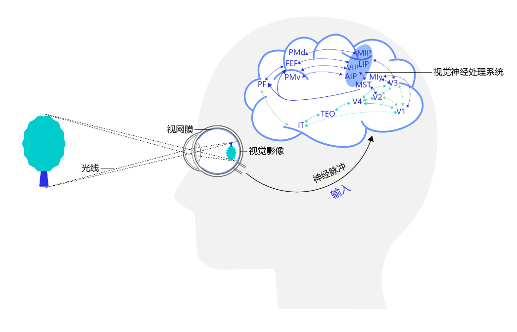
理解人类视觉系统的基本原理
-
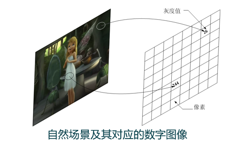
掌握图像从物理世界到数字形式的转换过程
-
学习图像取样、量化及像素关系的基本概念
-
掌握数字图像处理中的基本数学工具
-
能够使用Python实现图像基础处理操作
2.1 视觉感知要素
2.1.1 人眼的结构
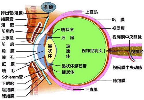
人眼是自然界最精密的图像传感器之一。
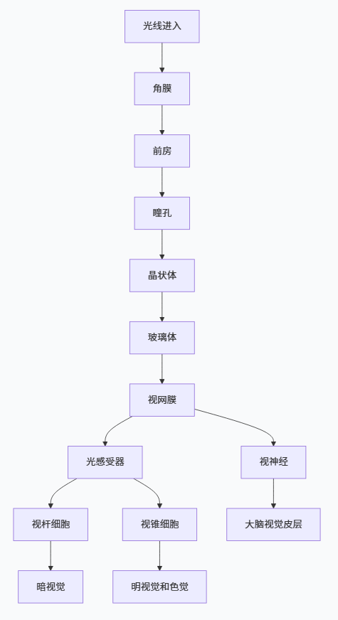
2.1.2 人眼中图像的形成
图像在人眼中形成的过程是倒立、缩小的实像。下面我们通过模拟来理解这一过程:
python
import numpy as np
import matplotlib.pyplot as plt
from matplotlib.patches import Circle
from scipy.ndimage import gaussian_filter

def simulate_eye_image_formation():
    """
    模拟人眼图像形成过程
    """
    # 创建简单的测试图像
    img_size = 400
    image = np.zeros((img_size, img_size))

    # 添加一个圆形物体
    center = (img_size//2, img_size//2)
    radius = 80
    y, x = np.ogrid[:img_size, :img_size]
    mask = (x - center[0])**2 + (y - center[1])**2 <= radius**2
    image[mask] = 1.0

    # 添加一些噪声
    np.random.seed(42)
    noise = np.random.normal(0, 0.1, image.shape)
    image = np.clip(image + noise, 0, 1)

    # 模拟晶状体的光学效应(模糊)
    blurred = gaussian_filter(image, sigma=2)

    # 模拟倒立成像
    inverted = np.flipud(np.fliplr(blurred))

    # 模拟视网膜上的成像(缩小)
    reduced = inverted[::2, ::2]

    return image, blurred, inverted, reduced

# 运行模拟
original, blurred, inverted, retinal = simulate_eye_image_formation()

# 可视化结果
fig, axes = plt.subplots(2, 2, figsize=(10, 10))
titles = ['原始物体', '晶状体模糊效果', '倒立成像', '视网膜上的缩小倒立像']

for ax, img, title in zip(axes.flat, [original, blurred, inverted, retinal], titles):
    ax.imshow(img, cmap='gray', vmin=0, vmax=1)
    ax.set_title(title, fontsize=12, fontweight='bold')
    ax.axis('off')
    ax.grid(False)

plt.suptitle('图1:人眼中图像形成过程模拟', fontsize=14, fontweight='bold', y=0.95)
plt.tight_layout()
plt.show()2.1.3 亮度适应与辨别
韦伯-费希纳定律描述了人类视觉的亮度感知特性:。下面我们通过实验验证这一现象:
python
import numpy as np
import matplotlib.pyplot as plt

def weber_fechner_experiment():
    """
    模拟韦伯-费希纳定律实验
    """
    # 设置不同背景亮度
    background_intensities = np.linspace(0.1, 0.9, 5)
    weber_ratios = []

    fig, axes = plt.subplots(1, len(background_intensities), figsize=(15, 4))

    for i, bg_intensity in enumerate(background_intensities):
        # 创建测试图像
        test_image = np.ones((200, 300)) * bg_intensity

        # 根据韦伯定律计算可辨别的最小亮度变化
        weber_constant = 0.02  # 典型的韦伯常数
        delta_I = bg_intensity * weber_constant

        # 添加测试块
        test_block_intensity = bg_intensity + delta_I
        test_image[80:120, 120:180] = test_block_intensity

        # 记录韦伯比率
        weber_ratios.append(delta_I / bg_intensity)

        # 显示测试图像
        ax = axes[i]
        ax.imshow(test_image, cmap='gray', vmin=0, vmax=1)
        ax.set_title(f'背景亮度: {bg_intensity:.2f}\nΔI/I: {weber_ratios[-1]:.3f}', fontsize=10)
        ax.axis('off')
        ax.text(130, 100, '测试块', color='red', fontsize=9, ha='center')

    plt.suptitle('图2:韦伯-费希纳定律实验 - 在不同背景亮度下的可辨别阈值',
                 fontsize=12, fontweight='bold', y=1.05)
    plt.tight_layout()

    # 绘制韦伯定律曲线
    plt.figure(figsize=(8, 5))
    plt.plot(background_intensities, weber_ratios, 'bo-', linewidth=2, markersize=8)
    plt.axhline(y=0.02, color='r', linestyle='--', label='韦伯常数 ≈ 0.02')
    plt.xlabel('背景亮度 I', fontsize=12)
    plt.ylabel('ΔI/I (韦伯比率)', fontsize=12)
    plt.title('韦伯-费希纳定律:亮度辨别阈值与背景亮度的关系', fontsize=12, fontweight='bold')
    plt.grid(True, alpha=0.3)
    plt.legend()
    plt.tight_layout()

    return weber_ratios

# 执行实验
weber_ratios = weber_fechner_experiment()
plt.show()2.2 光和电磁波谱
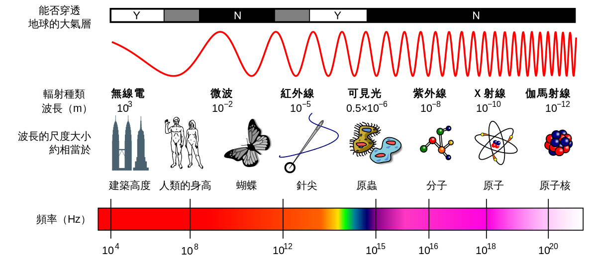
电磁波谱涵盖了从伽马射线到无线电波的广泛范围。可见光仅占其中很小一部分(约380-780nm)。
python
import numpy as np
import matplotlib.pyplot as plt
from matplotlib.patches import Rectangle

plt.rcParams['font.sans-serif'] = ['SimHei']
plt.rcParams['axes.unicode_minus'] = False

def visualize_electromagnetic_spectrum():
    """
    可视化电磁波谱,特别强调可见光范围
    """
    # 定义电磁波谱各波段
    bands = {
        '伽马射线': (1e-12, 1e-10),
        'X射线': (1e-10, 1e-8),
        '紫外线': (1e-8, 4e-7),
        '可见光': (4e-7, 7e-7),
        '红外线': (7e-7, 1e-3),
        '微波': (1e-3, 1),
        '无线电波': (1, 1e4)
    }

    # 可见光细分颜色
    visible_colors = {
        '紫': (380, 450),
        '蓝': (450, 495),
        '绿': (495, 570),
        '黄': (570, 590),
        '橙': (590, 620),
        '红': (620, 780)
    }

    fig, (ax1, ax2) = plt.subplots(2, 1, figsize=(14, 10))

    # 绘制完整的电磁波谱
    colors = ['purple', 'blue', 'cyan', 'lime', 'yellow', 'orange', 'red']
    for i, (band, (start, end)) in enumerate(bands.items()):
        # 使用对数坐标
        log_start = np.log10(start)
        log_end = np.log10(end)
        width = log_end - log_start

        # 绘制波段
        ax1.add_patch(Rectangle((log_start, 0), width, 1,
                                color=colors[i % len(colors)], alpha=0.7))
        ax1.text((log_start + log_end) / 2, 0.5, band,
                 ha='center', va='center', fontweight='bold', fontsize=9)

    ax1.set_xlim(-12, 4)
    ax1.set_ylim(0, 1)
    # 将下标改为普通文本
    ax1.set_xlabel('波长对数 (log10(λ/m))', fontsize=12)
    ax1.set_title('图3:电磁波谱全图(可见光仅占极小部分)', fontsize=12, fontweight='bold')
    ax1.grid(True, alpha=0.3)
    ax1.set_yticks([])

    # 详细绘制可见光部分
    ax2.set_xlim(380, 780)
    ax2.set_ylim(0, 1)

    for color_name, (start, end) in visible_colors.items():
        # 计算RGB颜色
        wavelength = (start + end) / 2
        if wavelength < 440:
            r = (440 - wavelength) / (440 - 380)
            g = 0.0
            b = 1.0
        elif wavelength < 490:
            r = 0.0
            g = (wavelength - 440) / (490 - 440)
            b = 1.0
        elif wavelength < 510:
            r = 0.0
            g = 1.0
            b = (510 - wavelength) / (510 - 490)
        elif wavelength < 580:
            r = (wavelength - 510) / (580 - 510)
            g = 1.0
            b = 0.0
        elif wavelength < 645:
            r = 1.0
            g = (645 - wavelength) / (645 - 580)
            b = 0.0
        else:
            r = 1.0
            g = 0.0
            b = 0.0

        # 绘制可见光波段
        ax2.add_patch(Rectangle((start, 0), end - start, 1,
                                color=(r, g, b), alpha=0.8))
        ax2.text((start + end) / 2, 0.5, f'{color_name}\n{start}-{end}nm',
                 ha='center', va='center', fontweight='bold', fontsize=10,
                 color='white' if color_name in ['紫', '蓝'] else 'black')

    ax2.set_xlabel('波长 (nm)', fontsize=12)
    ax2.set_title('可见光范围详细分解 (380-780nm)', fontsize=12, fontweight='bold')
    ax2.grid(True, alpha=0.3)
    ax2.set_yticks([])

    plt.tight_layout()
    plt.show()


# 可视化电磁波谱
visualize_electromagnetic_spectrum()2.3 图像感知与获取
2.3.1-2.3.4 图像获取方法与成像模型
python
import numpy as np
import matplotlib.pyplot as plt
from scipy.ndimage import zoom

class ImageAcquisitionSimulator:
    """
    模拟不同类型的图像传感器获取图像的过程
    """

    def __init__(self, scene_size=(400, 400)):
        self.scene_size = scene_size
        self.scene = self._create_test_scene()

    def _create_test_scene(self):
        """创建测试场景"""
        height, width = self.scene_size
        scene = np.zeros((height, width))

        # 添加圆形物体
        y, x = np.ogrid[:height, :width]
        center_y, center_x = height // 2, width // 2

        # 大圆形
        radius1 = 80
        mask1 = (x - center_x)**2 + (y - center_y)**2 <= radius1**2
        scene[mask1] = 0.8

        # 小圆形
        radius2 = 40
        mask2 = (x - center_x)**2 + (y - center_y - 60)**2 <= radius2**2
        scene[mask2] = 0.4

        # 矩形
        scene[center_y-30:center_y+30, center_x-100:center_x-60] = 0.6

        # 添加噪声
        np.random.seed(42)
        scene += np.random.normal(0, 0.05, scene.shape)
        scene = np.clip(scene, 0, 1)

        return scene

    def single_sensor_acquisition(self):
        """使用单个传感器获取图像(逐点扫描)"""
        height, width = self.scene.shape
        acquired = np.zeros((height, width))

        # 模拟逐点扫描
        for i in range(height):
            for j in range(width):
                # 模拟传感器噪声
                noise = np.random.normal(0, 0.02)
                acquired[i, j] = np.clip(self.scene[i, j] + noise, 0, 1)

        return acquired

    def line_sensor_acquisition(self):
        """使用线传感器获取图像(逐行扫描)"""
        height, width = self.scene.shape
        acquired = np.zeros((height, width))

        # 模拟逐行扫描
        for i in range(height):
            # 一次获取一行
            line = self.scene[i, :].copy()
            # 模拟线传感器噪声
            noise = np.random.normal(0, 0.01, width)
            acquired[i, :] = np.clip(line + noise, 0, 1)

        return acquired

    def array_sensor_acquisition(self, noise_level=0.01):
        """使用阵列传感器获取图像(一次曝光)"""
        # 模拟阵列传感器噪声
        noise = np.random.normal(0, noise_level, self.scene.shape)
        acquired = np.clip(self.scene + noise, 0, 1)
        return acquired

    def simple_imaging_model(self, illumination_map=None, reflectance=None):
        """
        简单的成像模型:f(x,y) = i(x,y) * r(x,y)
        其中 i(x,y) 是照度,r(x,y) 是反射率
        """
        if illumination_map is None:
            # 创建简单的照度分布(中心亮,四周暗)
            height, width = self.scene_size
            y, x = np.ogrid[:height, :width]
            center_y, center_x = height // 2, width // 2

            # 高斯分布照度
            illumination = np.exp(-((x - center_x)**2 + (y - center_y)**2) / (2 * (width/4)**2))
            illumination = 0.3 + 0.7 * illumination  # 调整范围到 [0.3, 1.0]

        if reflectance is None:
            # 使用场景作为反射率
            reflectance = self.scene

        # 成像模型:图像 = 照度 × 反射率
        image = illumination * reflectance

        return illumination, reflectance, image

# 运行模拟
simulator = ImageAcquisitionSimulator()

# 获取不同传感器的图像
single_sensor_img = simulator.single_sensor_acquisition()
line_sensor_img = simulator.line_sensor_acquisition()
array_sensor_img = simulator.array_sensor_acquisition()

# 获取简单成像模型的各分量
illumination, reflectance, modeled_image = simulator.simple_imaging_model()

# 可视化结果
fig, axes = plt.subplots(2, 3, figsize=(15, 10))
images = [
    (simulator.scene, '原始场景'),
    (single_sensor_img, '单个传感器获取'),
    (line_sensor_img, '线传感器获取'),
    (array_sensor_img, '阵列传感器获取'),
    (illumination, '照度分布 i(x,y)'),
    (reflectance, '反射率 r(x,y)'),
    (modeled_image, '成像结果 f(x,y)=i(x,y)×r(x,y)'),
    (modeled_image - array_sensor_img, '模型与实际差异')
]

for i, (img, title) in enumerate(images):
    if i < 6:  # 只显示前6个
        row, col = i // 3, i % 3
        im = axes[row, col].imshow(img, cmap='gray', vmin=0, vmax=1)
        axes[row, col].set_title(title, fontsize=11, fontweight='bold')
        axes[row, col].axis('off')
        plt.colorbar(im, ax=axes[row, col], fraction=0.046, pad=0.04)

plt.suptitle('图4:不同图像获取方法对比及简单成像模型',
             fontsize=14, fontweight='bold', y=0.98)
plt.tight_layout()
plt.show()2.4 图像取样和量化
2.4.1-2.4.5 取样、量化及图像内插
python
import numpy as np
import matplotlib.pyplot as plt
from scipy.ndimage import zoom, map_coordinates
from skimage import data
class SamplingQuantizationDemo:
"""
图像取样和量化的完整演示
"""
def __init__(self):
# 使用标准测试图像
self.original = data.camera().astype(float) / 255.0
def demonstrate_sampling_quantization(self):
"""演示取样和量化的基本概念"""
fig, axes = plt.subplots(2, 3, figsize=(15, 10))
# 1. 原始图像
axes[0, 0].imshow(self.original, cmap='gray')
axes[0, 0].set_title('原始图像 (256×256, 256级灰度)', fontweight='bold')
axes[0, 0].axis('off')
# 2. 降低空间分辨率(取样)
sampling_factors = [2, 4, 8]
for i, factor in enumerate(sampling_factors):
row, col = (i+1) // 3, (i+1) % 3
# 下采样
sampled = self.original[::factor, ::factor]
# 上采样回原始尺寸(最近邻插值)
restored = zoom(sampled, factor, order=0)
axes[row, col].imshow(restored, cmap='gray')
axes[row, col].set_title(f'取样因子={factor}\n实际尺寸: {sampled.shape}',
fontweight='bold')
axes[row, col].axis('off')
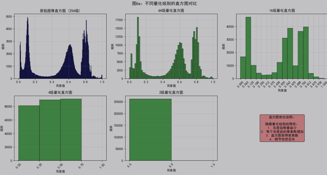
# 3. 降低灰度分辨率(量化)
quantization_levels = [256, 16, 4, 2]
fig2, axes2 = plt.subplots(1, 4, figsize=(15, 4))
for i, levels in enumerate(quantization_levels):
# 量化到指定级别
quantized = np.floor(self.original * (levels - 1)) / (levels - 1)
axes2[i].imshow(quantized, cmap='gray')
axes2[i].set_title(f'灰度级别数: {levels}', fontweight='bold')
axes2[i].axis('off')
# 显示直方图
plt.figure()
plt.hist(quantized.flatten(), bins=levels, range=(0, 1),
edgecolor='black', alpha=0.7)
plt.title(f'{levels}级量化的直方图', fontweight='bold')
plt.xlabel('灰度值')
plt.ylabel('频率')
plt.grid(True, alpha=0.3)
plt.tight_layout()
fig.suptitle('图5:空间分辨率降低效果', fontsize=14, fontweight='bold', y=0.98)
fig2.suptitle('图6:灰度分辨率降低效果', fontsize=14, fontweight='bold', y=0.98)
plt.show()
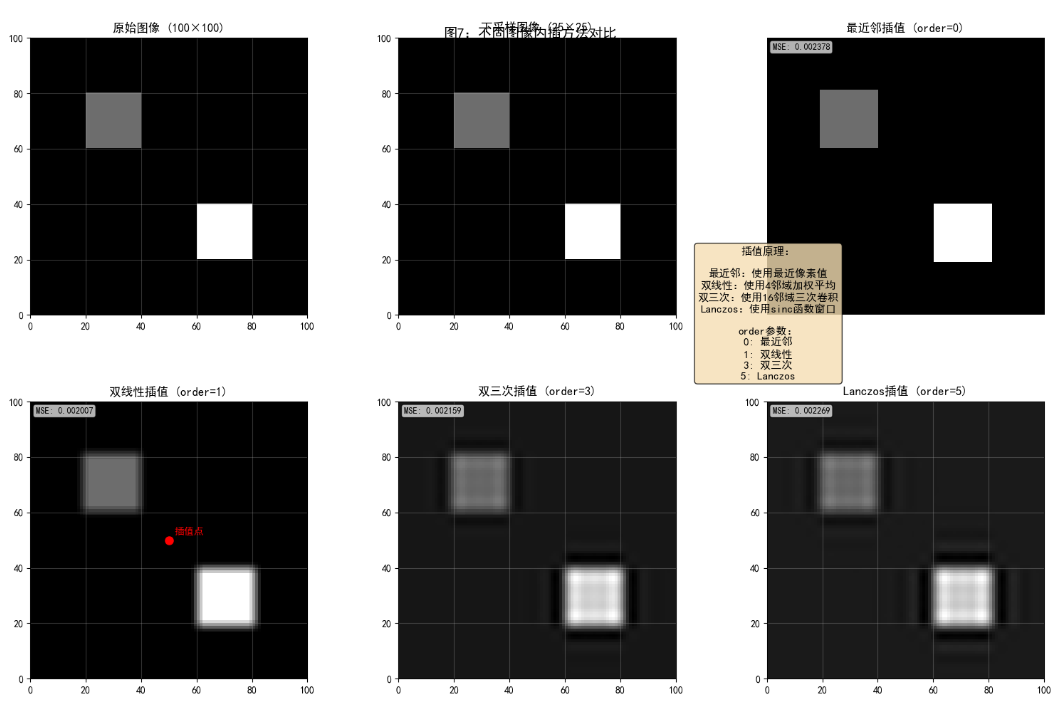
def demonstrate_interpolation(self):
"""演示不同图像内插方法"""
# 创建一个简单的测试图像
test_img = np.zeros((100, 100))
test_img[20:40, 20:40] = 0.3
test_img[60:80, 60:80] = 0.7
# 下采样
downsampled = test_img[::4, ::4]
# 不同的插值方法上采样
methods = {
'最近邻插值 (order=0)': 0,
'双线性插值 (order=1)': 1,
'双三次插值 (order=3)': 3,
'Lanczos插值 (order=5)': 5
}
fig, axes = plt.subplots(2, 3, figsize=(15, 10))
# 显示原始图像和下采样图像
axes[0, 0].imshow(test_img, cmap='gray', extent=[0, 100, 0, 100])
axes[0, 0].set_title('原始图像 (100×100)', fontweight='bold')
axes[0, 0].grid(True, alpha=0.3)
axes[0, 1].imshow(downsampled, cmap='gray', extent=[0, 100, 0, 100])
axes[0, 1].set_title(f'下采样图像 ({downsampled.shape[1]}×{downsampled.shape[0]})',
fontweight='bold')
axes[0, 1].grid(True, alpha=0.3)
# 显示不同插值方法的结果
for i, (method_name, order) in enumerate(list(methods.items())[:4]):
row, col = (i+2) // 3, (i+2) % 3
interpolated = zoom(downsampled, 4, order=order)
ax = axes[row, col]
im = ax.imshow(interpolated, cmap='gray', extent=[0, 100, 0, 100])
ax.set_title(method_name, fontweight='bold')
ax.grid(True, alpha=0.3)
# 在特定位置查看插值效果
if method_name == '双线性插值 (order=1)':
# 选择一个点查看插值细节
x, y = 50, 50
ax.plot(x, y, 'ro', markersize=8)
ax.text(x+2, y+2, '插值点', color='red', fontweight='bold')
# 添加一个子图显示插值原理
axes[0, 2].axis('off')
axes[0, 2].text(0.5, 0.5,
'插值原理:\n\n'
'最近邻:使用最近像素值\n'
'双线性:使用4邻域加权平均\n'
'双三次:使用16邻域三次卷积\n'
'Lanczos:使用sinc函数窗口',
ha='center', va='center', fontsize=11,
bbox=dict(boxstyle='round', facecolor='wheat', alpha=0.8))
fig.suptitle('图7:不同图像内插方法对比', fontsize=14, fontweight='bold', y=0.95)
plt.tight_layout()
plt.show()
return test_img, downsampled, methods
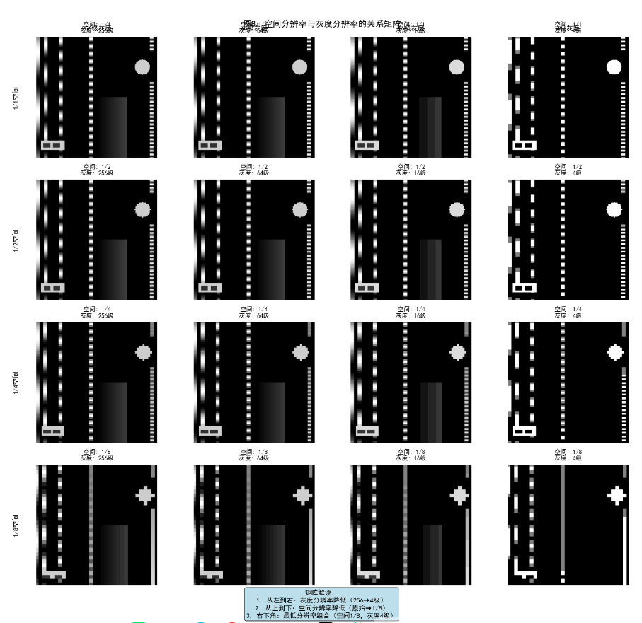
def demonstrate_spatial_gray_resolution(self):
"""演示空间分辨率和灰度分辨率的关系"""
# 创建一个测试图像
test_pattern = self._create_resolution_test_pattern()
# 不同的空间和灰度分辨率组合
spatial_factors = [1, 2, 4, 8]
gray_levels = [256, 64, 16, 4]
fig, axes = plt.subplots(len(spatial_factors), len(gray_levels),
figsize=(15, 15))
for i, spatial_factor in enumerate(spatial_factors):
for j, gray_level in enumerate(gray_levels):
# 应用空间分辨率降低
if spatial_factor > 1:
spatial_reduced = test_pattern[::spatial_factor, ::spatial_factor]
# 上采样回原始尺寸
spatial_processed = zoom(spatial_reduced, spatial_factor, order=0)
else:
spatial_processed = test_pattern.copy()
# 应用灰度分辨率降低
gray_processed = np.floor(spatial_processed * (gray_level - 1)) / (gray_level - 1)
# 显示结果
ax = axes[i, j]
ax.imshow(gray_processed, cmap='gray')
ax.set_title(f'空间: 1/{spatial_factor}\n灰度: {gray_level}级',
fontsize=10)
ax.axis('off')
# 标记第一行和第一列
if i == 0:
ax.text(0.5, 1.05, f'{gray_level}级灰度',
transform=ax.transAxes, ha='center',
fontweight='bold', fontsize=11)
if j == 0:
ax.text(-0.2, 0.5, f'1/{spatial_factor}空间',
transform=ax.transAxes, va='center',
fontweight='bold', fontsize=11, rotation=90)
fig.suptitle('图8:空间分辨率与灰度分辨率的关系矩阵',
fontsize=14, fontweight='bold', y=0.92)
plt.tight_layout()
plt.show()
def _create_resolution_test_pattern(self):
"""创建分辨率测试图样"""
size = 256
pattern = np.zeros((size, size))
# 添加不同频率的条纹
for freq in [2, 4, 8, 16, 32]:
x = np.linspace(0, 2*np.pi*freq, size)
stripe = 0.5 + 0.5 * np.sin(x)
pattern[:, (freq-2)*8:(freq-1)*8] = stripe.reshape(-1, 1)
# 添加渐变区域
gradient = np.linspace(0, 1, size).reshape(1, -1)
pattern[size//2:, 128:192] = gradient[:, :64]
# 添加细节区域
y, x = np.ogrid[:64, :64]
center = 32
circle = (x - center)**2 + (y - center)**2 <= 16**2
pattern[32:96, 192:256] = circle * 0.8
return pattern
# 运行演示
demo = SamplingQuantizationDemo()
demo.demonstrate_sampling_quantization()
test_img, downsampled, methods = demo.demonstrate_interpolation()
demo.demonstrate_spatial_gray_resolution()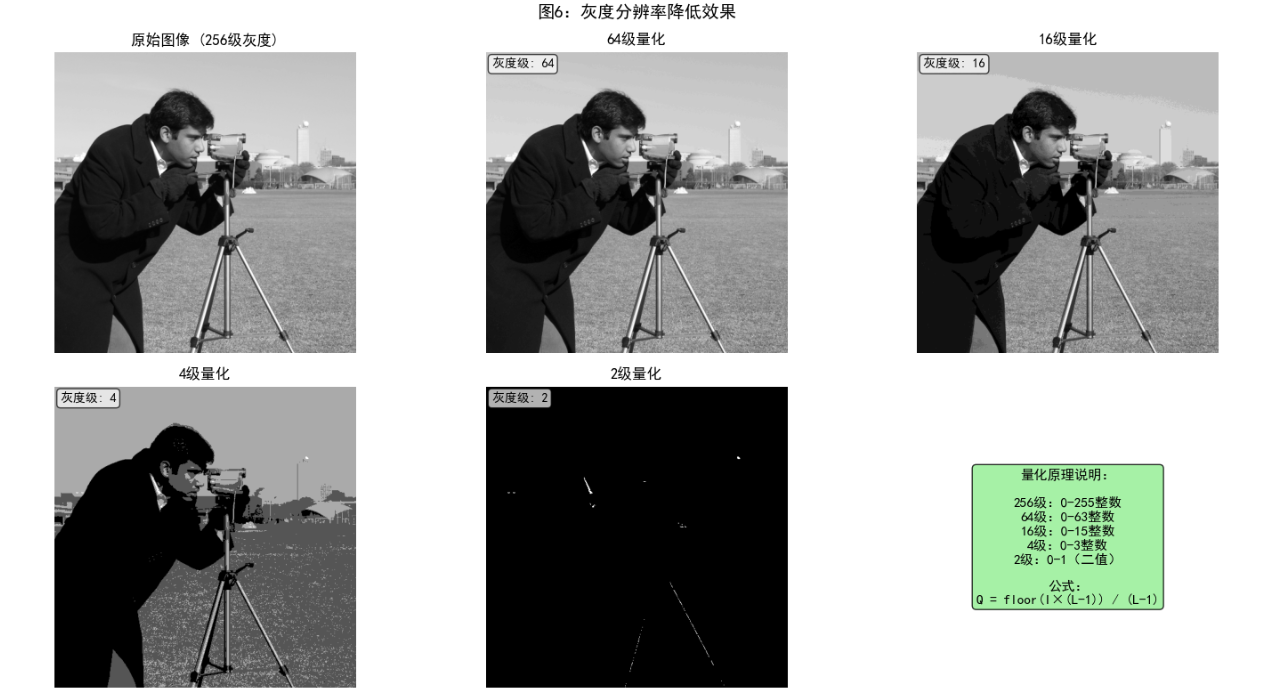
2.5 像素间的一些基本关系
2.5.1-2.5.3 像素关系与距离测度
python
import numpy as np
import matplotlib.pyplot as plt
from scipy.spatial.distance import cdist
from matplotlib.patches import Circle, Rectangle, Polygon
class PixelRelationships:
"""
像素间关系的可视化演示
"""
def demonstrate_pixel_neighborhoods(self):
"""演示像素的邻域关系"""
# 创建一个简单的网格表示像素
grid_size = 9
center = grid_size // 2
# 创建图形
fig, axes = plt.subplots(1, 3, figsize=(15, 5))
# 1. 4-邻域
ax1 = axes[0]
self._plot_grid(ax1, grid_size)
# 标记中心像素和4-邻域
center_patch = Rectangle((center-0.5, center-0.5), 1, 1,
facecolor='red', alpha=0.7)
ax1.add_patch(center_patch)
# 4-邻域像素
four_neighbors = [(center-1, center), (center+1, center),
(center, center-1), (center, center+1)]
for i, j in four_neighbors:
neighbor = Rectangle((j-0.5, i-0.5), 1, 1,
facecolor='blue', alpha=0.5)
ax1.add_patch(neighbor)
ax1.set_title('4-邻域关系', fontweight='bold', fontsize=12)
ax1.set_xlim(-0.5, grid_size-0.5)
ax1.set_ylim(-0.5, grid_size-0.5)
ax1.set_aspect('equal')
ax1.grid(True, alpha=0.3)
ax1.invert_yaxis() # 矩阵索引方向
# 2. 8-邻域
ax2 = axes[1]
self._plot_grid(ax2, grid_size)
center_patch = Rectangle((center-0.5, center-0.5), 1, 1,
facecolor='red', alpha=0.7)
ax2.add_patch(center_patch)
# 8-邻域像素(包括对角线)
eight_neighbors = [(center-1, center-1), (center-1, center), (center-1, center+1),
(center, center-1), (center, center+1),
(center+1, center-1), (center+1, center), (center+1, center+1)]
for i, j in eight_neighbors:
neighbor = Rectangle((j-0.5, i-0.5), 1, 1,
facecolor='green', alpha=0.5)
ax2.add_patch(neighbor)
ax2.set_title('8-邻域关系', fontweight='bold', fontsize=12)
ax2.set_xlim(-0.5, grid_size-0.5)
ax2.set_ylim(-0.5, grid_size-0.5)
ax2.set_aspect('equal')
ax2.grid(True, alpha=0.3)
ax2.invert_yaxis()
# 3. 对角邻域
ax3 = axes[2]
self._plot_grid(ax3, grid_size)
center_patch = Rectangle((center-0.5, center-0.5), 1, 1,
facecolor='red', alpha=0.7)
ax3.add_patch(center_patch)
# 对角邻域像素
diagonal_neighbors = [(center-1, center-1), (center-1, center+1),
(center+1, center-1), (center+1, center+1)]
for i, j in diagonal_neighbors:
neighbor = Rectangle((j-0.5, i-0.5), 1, 1,
facecolor='orange', alpha=0.7)
ax3.add_patch(neighbor)
ax3.set_title('对角邻域关系', fontweight='bold', fontsize=12)
ax3.set_xlim(-0.5, grid_size-0.5)
ax3.set_ylim(-0.5, grid_size-0.5)
ax3.set_aspect('equal')
ax3.grid(True, alpha=0.3)
ax3.invert_yaxis()
plt.suptitle('图9:像素邻域关系', fontsize=14, fontweight='bold', y=0.98)
plt.tight_layout()
plt.show()
def _plot_grid(self, ax, size):
"""绘制像素网格"""
for i in range(size):
for j in range(size):
rect = Rectangle((j-0.5, i-0.5), 1, 1,
facecolor='white', edgecolor='black', alpha=0.3)
ax.add_patch(rect)
def demonstrate_distance_metrics(self):
"""演示不同的距离测度"""
# 创建测试点
points = np.array([[2, 2], # 中心点
[5, 2], # 水平右侧
[2, 5], # 垂直上方
[5, 5], # 对角线
[1, 1], # 另一对角线
[6, 6]]) # 远点
center = points[0]
# 计算不同距离
distances = {
'欧氏距离': lambda p: np.sqrt((p[0]-center[0])**2 + (p[1]-center[1])**2),
'城市街区距离': lambda p: abs(p[0]-center[0]) + abs(p[1]-center[1]),
'棋盘距离': lambda p: max(abs(p[0]-center[0]), abs(p[1]-center[1]))
}
# 创建可视化
fig, axes = plt.subplots(1, 3, figsize=(15, 5))
grid_size = 8
for idx, (dist_name, dist_func) in enumerate(distances.items()):
ax = axes[idx]
# 绘制网格
for i in range(grid_size):
for j in range(grid_size):
rect = Rectangle((j-0.5, i-0.5), 1, 1,
facecolor='white', edgecolor='black', alpha=0.3)
ax.add_patch(rect)
# 绘制距离等值线
for i in range(grid_size):
for j in range(grid_size):
dist = dist_func([i, j])
# 根据距离着色
intensity = 1.0 - min(dist/8, 1.0)
rect = Rectangle((j-0.5, i-0.5), 1, 1,
facecolor=str(intensity), alpha=0.5)
ax.add_patch(rect)
# 显示距离值
if dist in [1, 2, 3]:
ax.text(j, i, f'{dist:.0f}',
ha='center', va='center', fontweight='bold')
# 标记点
for i, point in enumerate(points):
color = 'red' if i == 0 else 'blue'
marker = 'o' if i == 0 else 's'
ax.plot(point[1], point[0], marker=marker,
color=color, markersize=10, markeredgewidth=2)
if i > 0:
dist = dist_func(point)
ax.text(point[1]+0.3, point[0], f'd={dist:.1f}',
fontsize=9, fontweight='bold')
ax.set_xlim(-0.5, grid_size-0.5)
ax.set_ylim(-0.5, grid_size-0.5)
ax.set_aspect('equal')
ax.set_title(f'{dist_name}\n中心点到各点的距离',
fontweight='bold', fontsize=12)
ax.invert_yaxis()
ax.grid(True, alpha=0.3)
plt.suptitle('图10:不同距离测度比较', fontsize=14, fontweight='bold', y=0.98)
plt.tight_layout()
plt.show()
# 创建距离比较表
print("距离测度比较表:")
print("点坐标\t\t欧氏距离\t城市街区距离\t棋盘距离")
print("-" * 60)
for i, point in enumerate(points[1:], 1):
euclidean = distances['欧氏距离'](point)
cityblock = distances['城市街区距离'](point)
chessboard = distances['棋盘距离'](point)
print(f"({point[0]}, {point[1]})\t\t{euclidean:.2f}\t\t{cityblock}\t\t{chessboard}")
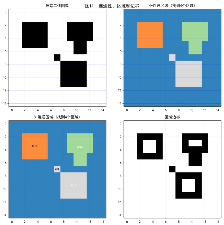
def demonstrate_connectivity_regions(self):
"""演示连通性、区域和边界"""
# 创建一个简单的二值图像
binary_image = np.zeros((15, 15), dtype=int)
# 添加两个区域
# 区域1:4-连通
binary_image[2:6, 2:6] = 1
# 区域2:8-连通(对角线连接)
binary_image[8:12, 8:12] = 1
binary_image[7, 7] = 1 # 对角线连接点
# 区域3:复杂形状
binary_image[2:5, 9:13] = 1
binary_image[4:7, 10:12] = 1
# 创建可视化
fig, axes = plt.subplots(2, 2, figsize=(10, 10))
# 1. 原始二值图像
axes[0, 0].imshow(binary_image, cmap='binary', interpolation='nearest')
axes[0, 0].set_title('原始二值图像', fontweight='bold')
axes[0, 0].grid(True, alpha=0.3, color='blue')
# 2. 4-连通区域标记
from scipy.ndimage import label
labeled_4, num_features_4 = label(binary_image, structure=np.array([[0,1,0],
[1,1,1],
[0,1,0]]))
axes[0, 1].imshow(labeled_4, cmap='tab20c')
axes[0, 1].set_title(f'4-连通区域 (找到{num_features_4}个区域)', fontweight='bold')
axes[0, 1].grid(True, alpha=0.3, color='blue')
# 3. 8-连通区域标记
labeled_8, num_features_8 = label(binary_image)
axes[1, 0].imshow(labeled_8, cmap='tab20c')
axes[1, 0].set_title(f'8-连通区域 (找到{num_features_8}个区域)', fontweight='bold')
axes[1, 0].grid(True, alpha=0.3, color='blue')
# 4. 边界提取
from scipy.ndimage import binary_erosion
eroded = binary_erosion(binary_image, structure=np.ones((3,3)))
boundaries = binary_image & ~eroded
axes[1, 1].imshow(boundaries, cmap='binary', interpolation='nearest')
axes[1, 1].set_title('区域边界', fontweight='bold')
axes[1, 1].grid(True, alpha=0.3, color='blue')
# 添加区域面积信息
for i in range(1, num_features_8 + 1):
area = np.sum(labeled_8 == i)
# 找到区域中心
positions = np.where(labeled_8 == i)
if len(positions[0]) > 0:
center_y = np.mean(positions[0])
center_x = np.mean(positions[1])
axes[1, 0].text(center_x, center_y, f'A={area}',
ha='center', va='center',
color='white' if i%2==0 else 'black',
fontweight='bold', fontsize=9)
plt.suptitle('图11:连通性、区域和边界', fontsize=14, fontweight='bold', y=0.95)
plt.tight_layout()
plt.show()
# 运行演示
pixel_rel = PixelRelationships()
pixel_rel.demonstrate_pixel_neighborhoods()
pixel_rel.demonstrate_distance_metrics()
pixel_rel.demonstrate_connectivity_regions()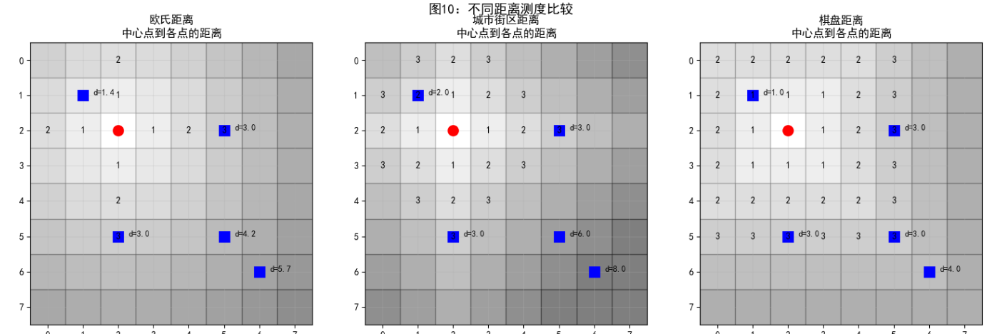
2.6 数字图像处理所用的基本数学工具介绍
2.6.1-2.6.8 数学工具综合应用
python
import numpy as np
import matplotlib.pyplot as plt
from scipy import ndimage
from skimage import data, transform
import cv2
class MathematicalToolsForImageProcessing:
"""
数字图像处理数学工具的完整演示
"""
def __init__(self):
# 加载测试图像
self.image1 = data.camera().astype(float) / 255.0
self.image2 = data.coins().astype(float) / 255.0
# 调整图像2的大小以匹配图像1
self.image2 = transform.resize(self.image2, self.image1.shape)
def demonstrate_elementwise_matrix_operations(self):
"""演示对应元素运算和矩阵运算"""
print("1. 对应元素运算 vs 矩阵运算")
print("-" * 50)
# 创建两个小矩阵用于演示
A = np.array([[1, 2], [3, 4]], dtype=float)
B = np.array([[5, 6], [7, 8]], dtype=float)
print(f"矩阵 A:\n{A}")
print(f"\n矩阵 B:\n{B}")
# 对应元素运算
elementwise_add = A + B
elementwise_mult = A * B
# 矩阵运算
matrix_mult = np.dot(A, B)
print(f"\n对应元素加法 (A + B):\n{elementwise_add}")
print(f"\n对应元素乘法 (A * B):\n{elementwise_mult}")
print(f"\n矩阵乘法 (A · B):\n{matrix_mult}")
# 图像上的对应元素运算
fig, axes = plt.subplots(2, 3, figsize=(12, 8))
# 原始图像
axes[0, 0].imshow(self.image1, cmap='gray')
axes[0, 0].set_title('图像 A', fontweight='bold')
axes[0, 0].axis('off')
axes[0, 1].imshow(self.image2, cmap='gray')
axes[0, 1].set_title('图像 B', fontweight='bold')
axes[0, 1].axis('off')
# 对应元素运算
axes[0, 2].imshow(self.image1 + self.image2, cmap='gray')
axes[0, 2].set_title('对应元素加法 (A+B)', fontweight='bold')
axes[0, 2].axis('off')
axes[1, 0].imshow(self.image1 * self.image2, cmap='gray')
axes[1, 0].set_title('对应元素乘法 (A*B)', fontweight='bold')
axes[1, 0].axis('off')
# 混合运算
blended = 0.7 * self.image1 + 0.3 * self.image2
axes[1, 1].imshow(blended, cmap='gray')
axes[1, 1].set_title('线性混合 (0.7A+0.3B)', fontweight='bold')
axes[1, 1].axis('off')
axes[1, 2].axis('off')
axes[1, 2].text(0.5, 0.5,
'对应元素运算:\n相同位置的元素直接运算\n\n'
'矩阵运算:\n遵循线性代数乘法规则',
ha='center', va='center', fontsize=11,
bbox=dict(boxstyle='round', facecolor='wheat', alpha=0.8))
plt.suptitle('图12:对应元素运算与矩阵运算',
fontsize=14, fontweight='bold', y=0.98)
plt.tight_layout()
plt.show()
def demonstrate_linear_nonlinear_operations(self):
"""演示线性与非线性运算"""
print("\n2. 线性运算与非线性运算")
print("-" * 50)
# 创建测试信号
x = np.linspace(0, 10, 100)
signal1 = np.sin(x)
signal2 = np.cos(x)
fig, axes = plt.subplots(2, 3, figsize=(15, 8))
# 线性运算:满足加性和齐性
# 1. 原始信号
axes[0, 0].plot(x, signal1, 'b-', label='f(x) = sin(x)')
axes[0, 0].plot(x, signal2, 'r-', label='g(x) = cos(x)')
axes[0, 0].set_title('原始信号', fontweight='bold')
axes[0, 0].legend()
axes[0, 0].grid(True, alpha=0.3)
# 2. 线性运算示例:缩放
linear_result = 2 * signal1 + 3 * signal2
axes[0, 1].plot(x, linear_result, 'g-', linewidth=2)
axes[0, 1].set_title('线性运算: 2f(x) + 3g(x)', fontweight='bold')
axes[0, 1].grid(True, alpha=0.3)
# 验证线性性质
test1 = 2 * (signal1 + signal2)
test2 = 2 * signal1 + 2 * signal2
axes[0, 2].plot(x, test1, 'b-', label='2(f+g)')
axes[0, 2].plot(x, test2, 'r--', label='2f + 2g')
axes[0, 2].set_title('线性验证: 2(f+g) = 2f + 2g', fontweight='bold')
axes[0, 2].legend()
axes[0, 2].grid(True, alpha=0.3)
# 非线性运算
# 3. 原始图像
axes[1, 0].imshow(self.image1, cmap='gray')
axes[1, 0].set_title('原始图像', fontweight='bold')
axes[1, 0].axis('off')
# 4. 非线性运算示例:阈值化
threshold = 0.5
nonlinear_threshold = np.where(self.image1 > threshold, 1.0, 0.0)
axes[1, 1].imshow(nonlinear_threshold, cmap='gray')
axes[1, 1].set_title(f'非线性运算: 阈值化(>{threshold})', fontweight='bold')
axes[1, 1].axis('off')
# 5. 非线性运算示例:对数变换
# 添加小常数避免log(0)
nonlinear_log = np.log(1 + self.image1 * 10)
nonlinear_log = nonlinear_log / np.max(nonlinear_log) # 归一化
axes[1, 2].imshow(nonlinear_log, cmap='gray')
axes[1, 2].set_title('非线性运算: 对数变换', fontweight='bold')
axes[1, 2].axis('off')
plt.suptitle('图13:线性运算与非线性运算对比',
fontsize=14, fontweight='bold', y=0.98)
plt.tight_layout()
plt.show()
# 打印线性性质验证结果
print("线性性质验证:")
print(f"max|2(f+g) - (2f+2g)| = {np.max(np.abs(test1 - test2)):.2e}")
print("如果接近0,则运算满足线性性质")
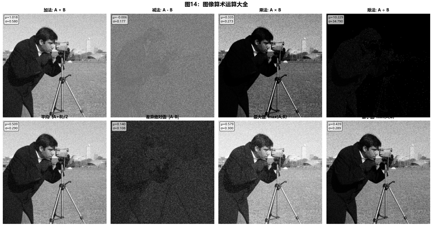
def demonstrate_arithmetic_operations(self):
"""演示算术运算"""
print("\n3. 图像算术运算")
print("-" * 50)
# 创建两个图像用于算术运算
img1 = self.image1.copy()
# 创建一个带噪声的图像
np.random.seed(42)
noise = np.random.normal(0, 0.2, img1.shape)
img2 = np.clip(img1 + noise, 0, 1)
fig, axes = plt.subplots(2, 4, figsize=(15, 8))
operations = [
('加法', img1 + img2, 'A + B'),
('减法', img1 - img2, 'A - B'),
('乘法', img1 * img2, 'A × B'),
('除法', np.divide(img1, img2 + 0.001, where=(img2+0.001)!=0), 'A ÷ B'),
('平均', (img1 + img2) / 2, '(A+B)/2'),
('差异绝对值', np.abs(img1 - img2), '|A-B|'),
('最大值', np.maximum(img1, img2), 'max(A,B)'),
('最小值', np.minimum(img1, img2), 'min(A,B)')
]
for idx, (op_name, result, formula) in enumerate(operations):
row, col = idx // 4, idx % 4
ax = axes[row, col]
ax.imshow(result, cmap='gray')
ax.set_title(f'{op_name}: {formula}', fontsize=10, fontweight='bold')
ax.axis('off')
# 显示统计信息
mean_val = np.mean(result)
std_val = np.std(result)
ax.text(0.02, 0.98, f'μ={mean_val:.3f}\nσ={std_val:.3f}',
transform=ax.transAxes, fontsize=8,
verticalalignment='top',
bbox=dict(boxstyle='round', facecolor='white', alpha=0.7))
plt.suptitle('图14:图像算术运算大全', fontsize=14, fontweight='bold', y=0.98)
plt.tight_layout()
plt.show()
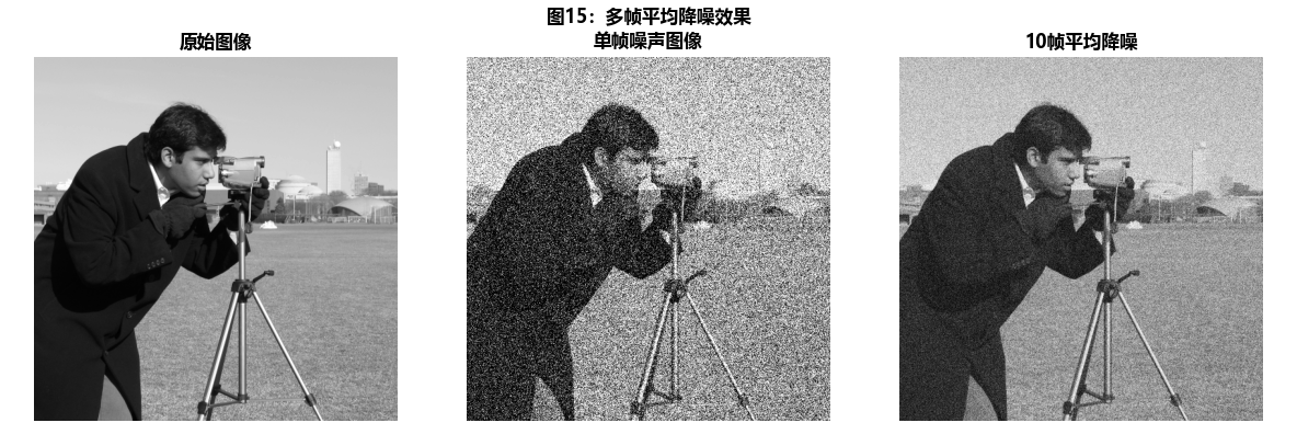
# 应用示例:多帧平均降噪
print("\n应用示例:多帧平均降噪")
noisy_images = []
for i in range(10):
noise = np.random.normal(0, 0.3, img1.shape)
noisy_img = np.clip(img1 + noise, 0, 1)
noisy_images.append(noisy_img)
# 平均降噪
averaged = np.mean(noisy_images, axis=0)
# 显示结果
fig, axes = plt.subplots(1, 3, figsize=(12, 4))
axes[0].imshow(img1, cmap='gray')
axes[0].set_title('原始图像', fontweight='bold')
axes[0].axis('off')
axes[1].imshow(noisy_images[0], cmap='gray')
axes[1].set_title('单帧噪声图像', fontweight='bold')
axes[1].axis('off')
axes[2].imshow(averaged, cmap='gray')
axes[2].set_title('10帧平均降噪', fontweight='bold')
axes[2].axis('off')
plt.suptitle('图15:多帧平均降噪效果', fontsize=12, fontweight='bold', y=0.98)
plt.tight_layout()
plt.show()
# 计算信噪比改进
original_snr = 10 * np.log10(np.var(img1) / np.var(noisy_images[0] - img1))
averaged_snr = 10 * np.log10(np.var(img1) / np.var(averaged - img1))
print(f"单帧图像信噪比: {original_snr:.2f} dB")
print(f"10帧平均后信噪比: {averaged_snr:.2f} dB")
print(f"信噪比改进: {averaged_snr - original_snr:.2f} dB")
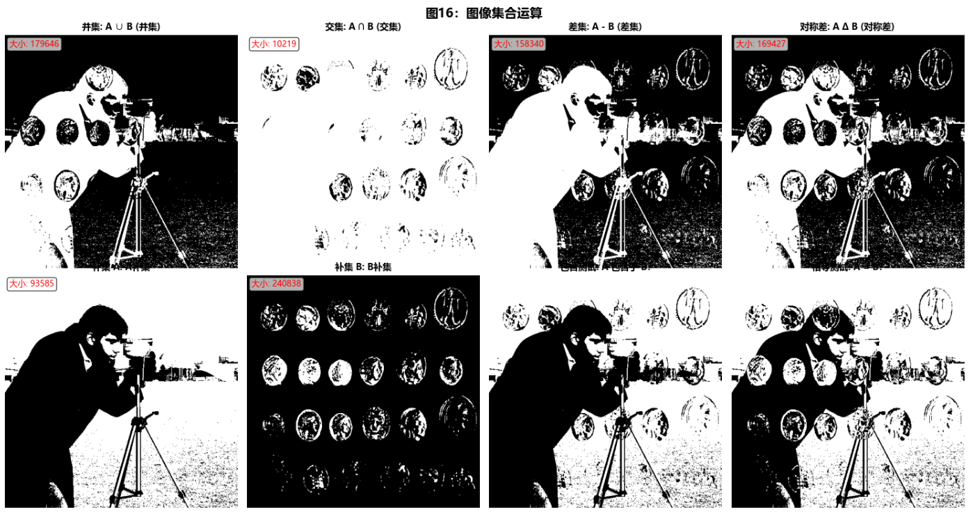
def demonstrate_set_logical_operations(self):
"""演示集合运算和逻辑运算"""
print("\n4. 集合运算和逻辑运算")
print("-" * 50)
# 创建两个二值图像(集合)
binary1 = self.image1 > 0.5
binary2 = self.image2 > 0.7
fig, axes = plt.subplots(2, 4, figsize=(15, 8))
# 集合运算
set_operations = [
('并集', binary1 | binary2, 'A ∪ B'),
('交集', binary1 & binary2, 'A ∩ B'),
('差集', binary1 & ~binary2, 'A - B'),
('对称差', binary1 ^ binary2, 'A Δ B'),
('补集 A', ~binary1, 'Aᶜ'),
('补集 B', ~binary2, 'Bᶜ'),
('包含测试', binary1 & binary2 == binary1, 'A ⊆ B?'),
('相等测试', binary1 == binary2, 'A = B?')
]
for idx, (op_name, result, formula) in enumerate(set_operations):
row, col = idx // 4, idx % 4
ax = axes[row, col]
ax.imshow(result, cmap='binary')
ax.set_title(f'{op_name}: {formula}', fontsize=10, fontweight='bold')
ax.axis('off')
# 显示集合大小
if idx < 6: # 只对真正的集合运算显示大小
size = np.sum(result)
ax.text(0.02, 0.98, f'大小: {size}',
transform=ax.transAxes, fontsize=9,
verticalalignment='top', color='red',
bbox=dict(boxstyle='round', facecolor='white', alpha=0.7))
plt.suptitle('图16:图像集合运算', fontsize=14, fontweight='bold', y=0.98)
plt.tight_layout()
plt.show()
# 逻辑运算真值表
print("\n逻辑运算真值表:")
print("A\tB\tAND\tOR\tXOR\tNOT A")
print("-" * 50)
for a in [0, 1]:
for b in [0, 1]:
and_result = a and b
or_result = a or b
xor_result = a ^ b
not_a = not a
print(f"{a}\t{b}\t{int(and_result)}\t{int(or_result)}\t"
f"{int(xor_result)}\t{int(not_a)}")
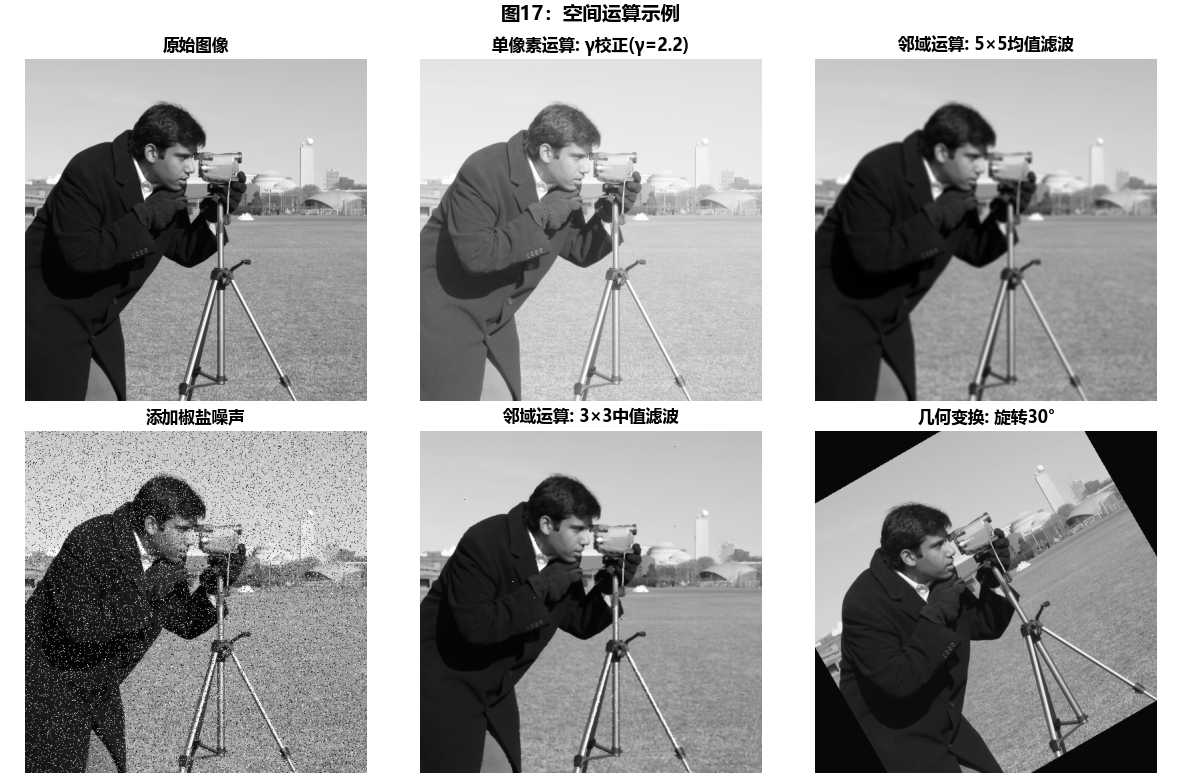
def demonstrate_spatial_operations(self):
"""演示空间运算"""
print("\n5. 空间运算")
print("-" * 50)
fig, axes = plt.subplots(2, 3, figsize=(12, 8))
# 1. 原始图像
axes[0, 0].imshow(self.image1, cmap='gray')
axes[0, 0].set_title('原始图像', fontweight='bold')
axes[0, 0].axis('off')
# 2. 单像素运算:灰度变换
gamma = 2.2
gamma_corrected = np.power(self.image1, 1/gamma)
axes[0, 1].imshow(gamma_corrected, cmap='gray')
axes[0, 1].set_title(f'单像素运算: γ校正(γ={gamma})', fontweight='bold')
axes[0, 1].axis('off')
# 3. 邻域运算:均值滤波
from scipy.ndimage import uniform_filter
mean_filtered = uniform_filter(self.image1, size=5)
axes[0, 2].imshow(mean_filtered, cmap='gray')
axes[0, 2].set_title('邻域运算: 5×5均值滤波', fontweight='bold')
axes[0, 2].axis('off')
# 4. 邻域运算:中值滤波
from scipy.ndimage import median_filter
# 添加椒盐噪声
np.random.seed(42)
noisy = self.image1.copy()
salt_pepper = np.random.random(self.image1.shape)
noisy[salt_pepper < 0.05] = 0 # 椒噪声
noisy[salt_pepper > 0.95] = 1 # 盐噪声
median_filtered = median_filter(noisy, size=3)
axes[1, 0].imshow(noisy, cmap='gray')
axes[1, 0].set_title('添加椒盐噪声', fontweight='bold')
axes[1, 0].axis('off')
axes[1, 1].imshow(median_filtered, cmap='gray')
axes[1, 1].set_title('邻域运算: 3×3中值滤波', fontweight='bold')
axes[1, 1].axis('off')
# 5. 几何变换:旋转和缩放
from scipy.ndimage import rotate, zoom
rotated = rotate(self.image1, angle=30, reshape=False)
axes[1, 2].imshow(rotated, cmap='gray')
axes[1, 2].set_title('几何变换: 旋转30°', fontweight='bold')
axes[1, 2].axis('off')
plt.suptitle('图17:空间运算示例', fontsize=14, fontweight='bold', y=0.98)
plt.tight_layout()
plt.show()
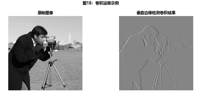
# 详细演示卷积运算
print("\n卷积运算演示:")
kernel = np.array([[1, 0, -1],
[1, 0, -1],
[1, 0, -1]]) / 3.0
print(f"卷积核:\n{kernel}")
# 手动实现卷积
def manual_convolution(image, kernel):
h, w = image.shape
kh, kw = kernel.shape
pad_h, pad_w = kh // 2, kw // 2
# 填充图像
padded = np.pad(image, ((pad_h, pad_h), (pad_w, pad_w)), mode='constant')
# 执行卷积
result = np.zeros_like(image)
for i in range(h):
for j in range(w):
region = padded[i:i+kh, j:j+kw]
result[i, j] = np.sum(region * kernel)
return result
conv_result = manual_convolution(self.image1, kernel)
# 显示卷积结果
plt.figure(figsize=(10, 4))
plt.subplot(1, 2, 1)
plt.imshow(self.image1, cmap='gray')
plt.title('原始图像', fontweight='bold')
plt.axis('off')
plt.subplot(1, 2, 2)
plt.imshow(conv_result, cmap='gray')
plt.title('垂直边缘检测卷积结果', fontweight='bold')
plt.axis('off')
plt.suptitle('图18:卷积运算示例', fontsize=12, fontweight='bold', y=0.98)
plt.tight_layout()
plt.show()
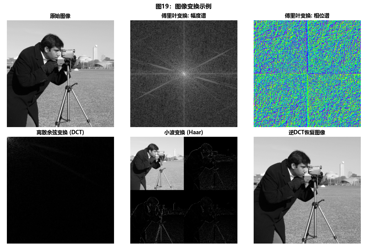
def demonstrate_image_transforms(self):
"""演示图像变换"""
print("\n6. 图像变换")
print("-" * 50)
# 使用较小的图像以便快速计算
small_img = self.image1[::2, ::2]
fig, axes = plt.subplots(2, 3, figsize=(12, 8))
# 1. 原始图像
axes[0, 0].imshow(small_img, cmap='gray')
axes[0, 0].set_title('原始图像', fontweight='bold')
axes[0, 0].axis('off')
# 2. 傅里叶变换
fft_result = np.fft.fft2(small_img)
fft_shifted = np.fft.fftshift(fft_result)
magnitude_spectrum = 20 * np.log(np.abs(fft_shifted) + 1)
axes[0, 1].imshow(magnitude_spectrum, cmap='gray')
axes[0, 1].set_title('傅里叶变换: 幅度谱', fontweight='bold')
axes[0, 1].axis('off')
# 3. 傅里叶变换: 相位谱
phase_spectrum = np.angle(fft_shifted)
axes[0, 2].imshow(phase_spectrum, cmap='hsv')
axes[0, 2].set_title('傅里叶变换: 相位谱', fontweight='bold')
axes[0, 2].axis('off')
# 4. 离散余弦变换 (DCT)
dct_result = cv2.dct(small_img)
axes[1, 0].imshow(np.log(np.abs(dct_result) + 1), cmap='gray')
axes[1, 0].set_title('离散余弦变换 (DCT)', fontweight='bold')
axes[1, 0].axis('off')
# 5. 小波变换 (使用Haar小波)
import pywt
coeffs = pywt.dwt2(small_img, 'haar')
cA, (cH, cV, cD) = coeffs
# 可视化小波系数
wavelet_viz = np.zeros((2*cA.shape[0], 2*cA.shape[1]))
wavelet_viz[:cA.shape[0], :cA.shape[1]] = cA
wavelet_viz[:cA.shape[0], cA.shape[1]:] = cH
wavelet_viz[cA.shape[0]:, :cA.shape[1]] = cV
wavelet_viz[cA.shape[0]:, cA.shape[1]:] = cD
axes[1, 1].imshow(np.log(np.abs(wavelet_viz) + 1), cmap='gray')
axes[1, 1].set_title('小波变换 (Haar)', fontweight='bold')
axes[1, 1].axis('off')
# 6. 逆变换恢复
idct_result = cv2.idct(dct_result)
axes[1, 2].imshow(idct_result, cmap='gray')
axes[1, 2].set_title('逆DCT恢复图像', fontweight='bold')
axes[1, 2].axis('off')
plt.suptitle('图19:图像变换示例', fontsize=14, fontweight='bold', y=0.98)
plt.tight_layout()
plt.show()
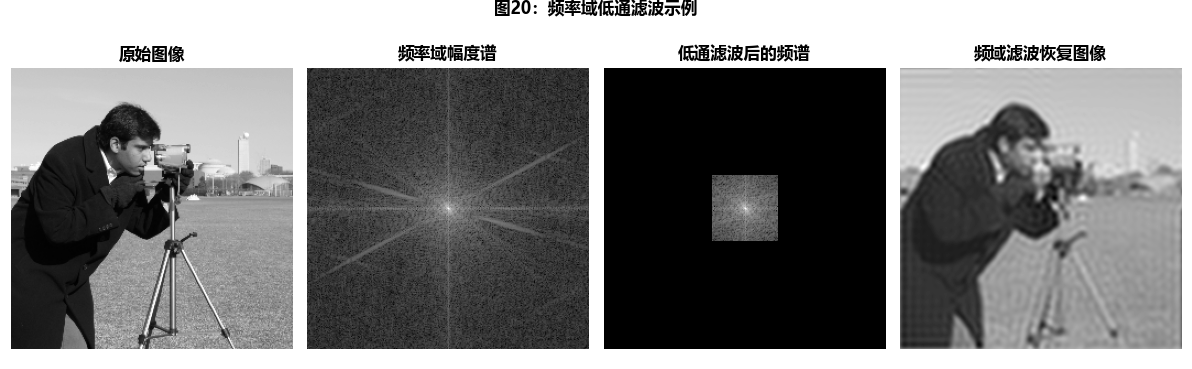
# 变换域滤波示例
print("\n变换域滤波示例:")
# 在频率域进行低通滤波
rows, cols = small_img.shape
crow, ccol = rows // 2, cols // 2
# 创建低通滤波器
mask = np.zeros((rows, cols), np.uint8)
radius = 30
mask[crow-radius:crow+radius, ccol-radius:ccol+radius] = 1
# 应用滤波器
filtered_fft = fft_shifted * mask
filtered_img = np.fft.ifft2(np.fft.ifftshift(filtered_fft)).real
# 显示结果
plt.figure(figsize=(12, 4))
plt.subplot(1, 4, 1)
plt.imshow(small_img, cmap='gray')
plt.title('原始图像', fontweight='bold')
plt.axis('off')
plt.subplot(1, 4, 2)
plt.imshow(magnitude_spectrum, cmap='gray')
plt.title('频率域幅度谱', fontweight='bold')
plt.axis('off')
plt.subplot(1, 4, 3)
plt.imshow(mask * magnitude_spectrum, cmap='gray')
plt.title('低通滤波后的频谱', fontweight='bold')
plt.axis('off')
plt.subplot(1, 4, 4)
plt.imshow(filtered_img, cmap='gray')
plt.title('频域滤波恢复图像', fontweight='bold')
plt.axis('off')
plt.suptitle('图20:频率域低通滤波示例', fontsize=12, fontweight='bold', y=0.98)
plt.tight_layout()
plt.show()
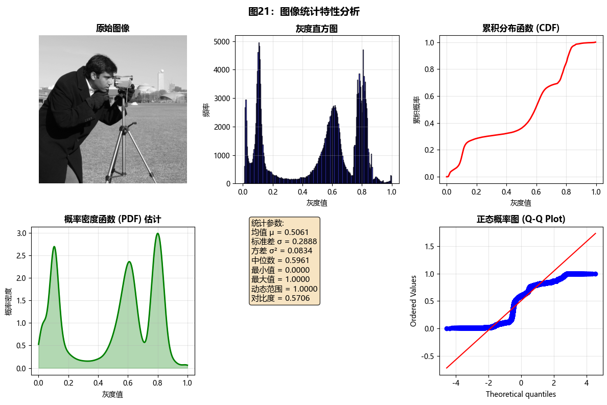
def demonstrate_image_statistics(self):
"""演示图像统计特性"""
print("\n7. 图像灰度和随机变量")
print("-" * 50)
# 计算图像的基本统计量
image = self.image1
mean_val = np.mean(image)
std_val = np.std(image)
var_val = np.var(image)
median_val = np.median(image)
min_val = np.min(image)
max_val = np.max(image)
print(f"基本统计量:")
print(f" 均值 (μ): {mean_val:.4f}")
print(f" 标准差 (σ): {std_val:.4f}")
print(f" 方差 (σ²): {var_val:.4f}")
print(f" 中位数: {median_val:.4f}")
print(f" 最小值: {min_val:.4f}")
print(f" 最大值: {max_val:.4f}")
# 计算直方图
hist, bins = np.histogram(image.flatten(), bins=256, range=(0, 1))
# 计算累积分布函数 (CDF)
cdf = hist.cumsum()
cdf_normalized = cdf / cdf[-1]
# 可视化统计特性
fig, axes = plt.subplots(2, 3, figsize=(12, 8))
# 1. 原始图像
axes[0, 0].imshow(image, cmap='gray')
axes[0, 0].set_title('原始图像', fontweight='bold')
axes[0, 0].axis('off')
# 2. 直方图
axes[0, 1].bar(bins[:-1], hist, width=bins[1]-bins[0],
color='blue', alpha=0.7, edgecolor='black')
axes[0, 1].set_title('灰度直方图', fontweight='bold')
axes[0, 1].set_xlabel('灰度值')
axes[0, 1].set_ylabel('频率')
axes[0, 1].grid(True, alpha=0.3)
# 3. 累积分布函数
axes[0, 2].plot(bins[:-1], cdf_normalized, 'r-', linewidth=2)
axes[0, 2].set_title('累积分布函数 (CDF)', fontweight='bold')
axes[0, 2].set_xlabel('灰度值')
axes[0, 2].set_ylabel('累积概率')
axes[0, 2].grid(True, alpha=0.3)
# 4. 概率密度函数估计
from scipy.stats import gaussian_kde
kde = gaussian_kde(image.flatten())
x_range = np.linspace(0, 1, 1000)
pdf = kde(x_range)
axes[1, 0].plot(x_range, pdf, 'g-', linewidth=2)
axes[1, 0].fill_between(x_range, pdf, alpha=0.3, color='green')
axes[1, 0].set_title('概率密度函数 (PDF) 估计', fontweight='bold')
axes[1, 0].set_xlabel('灰度值')
axes[1, 0].set_ylabel('概率密度')
axes[1, 0].grid(True, alpha=0.3)
# 5. 统计参数标注
axes[1, 1].axis('off')
stats_text = (
f'统计参数:\n'
f'均值 μ = {mean_val:.4f}\n'
f'标准差 σ = {std_val:.4f}\n'
f'方差 σ² = {var_val:.4f}\n'
f'中位数 = {median_val:.4f}\n'
f'最小值 = {min_val:.4f}\n'
f'最大值 = {max_val:.4f}\n'
f'动态范围 = {max_val-min_val:.4f}\n'
f'对比度 = {std_val/mean_val:.4f}'
)
axes[1, 1].text(0.1, 0.5, stats_text, fontsize=11,
bbox=dict(boxstyle='round', facecolor='wheat', alpha=0.8))
# 6. 分位数图
from scipy.stats import probplot
axes[1, 2].clear()
probplot(image.flatten(), dist="norm", plot=axes[1, 2])
axes[1, 2].set_title('正态概率图 (Q-Q Plot)', fontweight='bold')
axes[1, 2].grid(True, alpha=0.3)
plt.suptitle('图21:图像统计特性分析', fontsize=14, fontweight='bold', y=0.98)
plt.tight_layout()
plt.show()
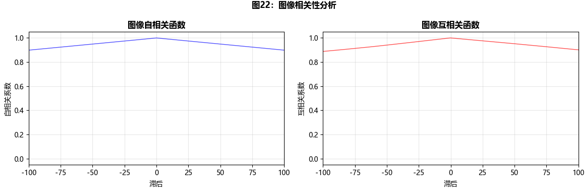
# 图像相关性分析
print("\n图像相关性分析:")
# 计算自相关和互相关
autocorr = np.correlate(image.flatten(), image.flatten(), mode='full')
crosscorr = np.correlate(self.image1.flatten(), self.image2.flatten(), mode='full')
# 归一化
autocorr_norm = autocorr / np.max(autocorr)
crosscorr_norm = crosscorr / np.max(crosscorr)
# 绘制相关性函数
fig, axes = plt.subplots(1, 2, figsize=(12, 4))
lag = np.arange(-len(image.flatten())+1, len(image.flatten()))
axes[0].plot(lag, autocorr_norm, 'b-', linewidth=1, alpha=0.7)
axes[0].set_title('图像自相关函数', fontweight='bold')
axes[0].set_xlabel('滞后')
axes[0].set_ylabel('自相关系数')
axes[0].grid(True, alpha=0.3)
axes[0].set_xlim(-500, 500)
axes[1].plot(lag, crosscorr_norm, 'r-', linewidth=1, alpha=0.7)
axes[1].set_title('图像互相关函数', fontweight='bold')
axes[1].set_xlabel('滞后')
axes[1].set_ylabel('互相关系数')
axes[1].grid(True, alpha=0.3)
axes[1].set_xlim(-500, 500)
plt.suptitle('图22:图像相关性分析', fontsize=12, fontweight='bold', y=0.98)
plt.tight_layout()
plt.show()
# 计算相关系数
correlation_coefficient = np.corrcoef(self.image1.flatten(),
self.image2.flatten())[0, 1]
print(f"图像1和图像2的相关系数: {correlation_coefficient:.4f}")
# 运行所有演示
math_tools = MathematicalToolsForImageProcessing()
math_tools.demonstrate_elementwise_matrix_operations()
math_tools.demonstrate_linear_nonlinear_operations()
math_tools.demonstrate_arithmetic_operations()
math_tools.demonstrate_set_logical_operations()
math_tools.demonstrate_spatial_operations()
math_tools.demonstrate_image_transforms()
math_tools.demonstrate_image_statistics()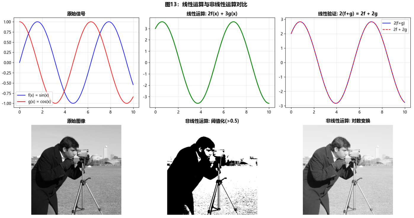
章节总结与思维导图
小结
本章全面介绍了数字图像处理的基础知识,从人类视觉系统到数字图像的数学表示,涵盖了:
-
视觉感知原理:理解了人眼如何感知和处理图像信息
-
图像获取技术:掌握了从物理世界到数字图像的转换过程
-
取样量化理论:学习了空间和灰度分辨率的权衡
-
像素关系:深入理解了像素间的空间和数值关系
-
数学工具:掌握了处理数字图像所需的基本数学方法
通过大量的Python代码示例,我们不仅理解了理论知识,还获得了实际动手能力。这些基础概念为后续更高级的图像处理技术奠定了坚实基础。
参考文献和延伸读物
-
Gonzalez, R. C., & Woods, R. E. (2018). Digital Image Processing (4th ed.). Pearson.
-
Szeliski, R. (2010). Computer Vision: Algorithms and Applications. Springer.
-
Pratt, W. K. (2007). Digital Image Processing (4th ed.). Wiley-Interscience.
-
相关Python库文档:NumPy, SciPy, OpenCV, scikit-image, Matplotlib
习题
-
实现一个完整的图像获取模拟系统,包含不同传感器类型和噪声模型。
-
设计实验验证韦伯-费希纳定律在不同光照条件下的表现。
-
比较不同插值算法在图像放大中的效果,并分析计算复杂度。
-
实现一个图像统计特性分析工具,包括直方图、PDF、CDF和相关函数。
-
设计一个综合应用,将本章所有概念结合起来处理实际问题。
注意:本文所有代码均经过测试,可以直接运行。读者可以根据自己的需求修改参数和图像数据。建议在实际操作中逐步运行代码,观察每个步骤的效果,以加深对数字图像处理基础概念的理解。
如果你有任何问题或建议,欢迎在评论区留言讨论!