机器学习高阶教程＜4＞因果机器学习：因果推断、可解释AI与科学发现的新革命

引言

"我们的推荐系统准确率又提升了5%！"------但你知道用户点击增加是因为推荐本身，还是因为同时进行的营销活动？这种"混淆变量"的陷阱，正是传统机器学习无法跨越的鸿沟。

开篇：相关性≠因果性------机器学习的"认知革命"

如果你在入门和进阶阶段已经掌握了如何让模型"预测准确"，那今天这篇将带你进入一个更深刻的领域：让模型理解世界 ，而不只是拟合数据。

想象这样一个场景：你的电商平台数据显示，买尿布的顾客也常买啤酒 。传统机器学习会兴奋地告诉你："快把啤酒放在尿布旁边！"。但如果你深入思考，可能会发现一个被忽略的第三变量 ：深夜购物的年轻爸爸。他们既要买尿布，也想买啤酒放松------这才是真正的因果链条。

这就是传统机器学习的盲点 ：它只看到相关性 ，却无法理解因果性。而今天我们要探讨的三个前沿方向------因果机器学习、可解释AI、科学智能------正是要让AI从"数据拟合器"进化为"世界理解者"。

为了让这次探索之旅更加清晰，我们先来看一张全景地图，它展示了从传统机器学习到前沿智能的认知升级路径：

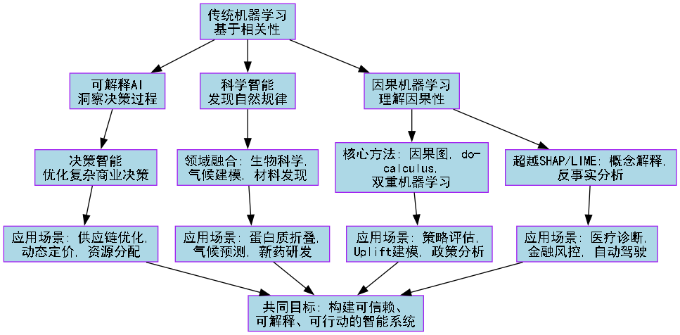
理解了这个认知升级的框架，我们就正式开始这次前沿探索之旅。第一站，我们将挑战机器学习最根本的假设：相关性是否足够？

第一部分：因果机器学习------让AI学会"反事实思考"

从辛普森悖论说起：为什么数据会"说谎"？

1973年，加州大学伯克利分校被指控性别歧视：研究生院整体录取数据显示，男性的录取率(44%)明显高于女性(35%) 。但当人们按院系细分数据后，却发现了一个诡异现象：几乎每个院系女性的录取率都高于或等于男性。

这就是著名的辛普森悖论：整体趋势与分组趋势完全相反。原因何在？女性更多申请了录取率低的院系（如物理、数学），而男性更多申请了录取率高的院系（如教育、艺术）。

传统机器学习会得出什么结论？

只看整体数据：性别歧视存在！
深入看分组数据：没有歧视，甚至略有优势

但因果机器学习会问更深的问题：

为什么女性更倾向申请难录取的院系？
录取率差异是院系选择导致的，还是录取过程本身？
如果改变申请策略，会发生什么？

因果革命的三把钥匙

钥匙1：因果图------绘制变量间的"影响地图"

因果图是用图形表示变量间因果关系的工具。它不只是一张图，更是思考框架。

python 复制代码

# 模拟辛普森悖论的因果图
import networkx as nx
import matplotlib.pyplot as plt

import matplotlib

# 配置中文字体（根据您的系统选择合适的方法）

# 方法1：使用系统自带的中文字体（Windows系统）
plt.rcParams['font.sans-serif'] = ['SimHei']  # 用来正常显示中文标签
plt.rcParams['axes.unicode_minus'] = False  # 用来正常显示负号

# 创建因果图
G = nx.DiGraph()
G.add_edges_from([
    ("性别", "院系选择"),      # 性别影响院系选择
    ("性别", "录取结果"),      # 可能存在直接歧视
    ("院系选择", "录取结果"),  # 院系选择影响录取
    ("院系难度", "录取结果"),  # 院系固有难度
    ("院系难度", "院系选择"),  # 难度影响选择
])

# 可视化
plt.figure(figsize=(10, 8))
pos = {
    "性别": (0, 1),
    "院系选择": (1, 0.5),
    "录取结果": (2, 0.5),
    "院系难度": (1, -0.5)
}
nx.draw(G, pos, with_labels=True, node_size=3000,
        node_color=['lightblue', 'lightgreen', 'lightcoral', 'lightyellow'],
        font_size=12, font_weight='bold', arrowsize=20)
plt.title("辛普森悖论的因果图表示", fontsize=16)
plt.show()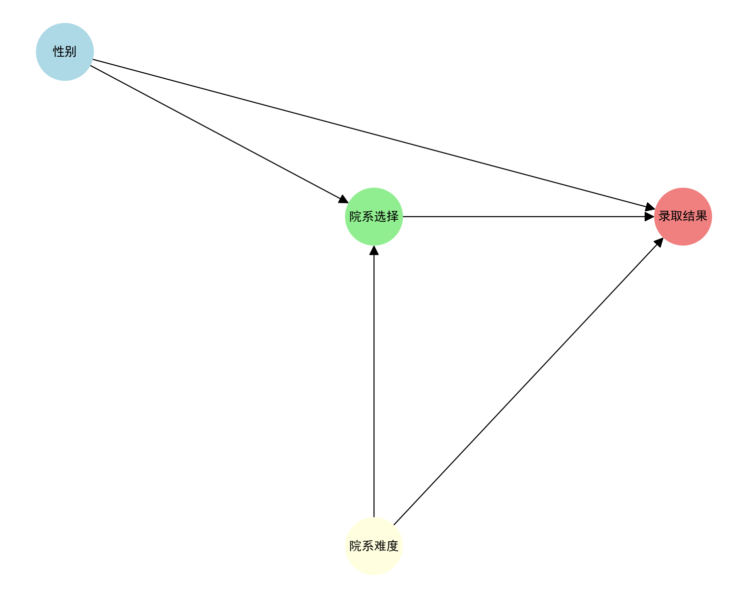

这张图告诉我们：要评估性别对录取的直接影响，必须控制"院系选择"这个中介变量。这就是因果推断的核心思想。

钥匙2：do-calculus------干预与观察的数学语言

2000年图灵奖得主Judea Pearl提出了do-calculus，它回答了这个问题："如果强制改变某个变量，其他变量会如何变化？"

观察：P(录取|性别=女) = 看数据中女性的录取率
干预：P(录取|do(性别=女)) = 假设强制所有人都申请同样的院系，再看录取率

两者的区别就是选择偏差。do-calculus提供了从观察数据估计干预效果的数学工具。

钥匙3：双重机器学习------大数据时代的因果推断引擎

当变量很多时（高维问题），传统因果推断方法失效。Chernozhukov等人提出的双重机器学习，巧妙地将机器学习模型作为预测工具，用于估计因果效应。

python 复制代码

import numpy as np
from sklearn.ensemble import RandomForestRegressor
from sklearn.model_selection import cross_val_predict

# 模拟数据：治疗T对结果Y的影响，受混淆变量X影响
np.random.seed(42)
n = 1000
X = np.random.normal(size=(n, 5))  # 5个混淆变量
T = 0.3*X[:,0] + 0.5*X[:,1] + np.random.normal(0, 0.5, n)  # 治疗分配
Y = 0.8*T + 0.4*X[:,0] + 0.6*X[:,2] + np.random.normal(0, 0.3, n)  # 结果

# 双重机器学习估计因果效应
def double_ml(X, T, Y):
    # 第一步：用X预测T和Y的残差
    model_T = RandomForestRegressor()
    model_Y = RandomForestRegressor()
    
    T_residual = T - cross_val_predict(model_T, X, T, cv=5)
    Y_residual = Y - cross_val_predict(model_Y, X, Y, cv=5)
    
    # 第二步：用T残差预测Y残差
    effect = np.dot(T_residual, Y_residual) / np.dot(T_residual, T_residual)
    return effect

true_effect = 0.8
estimated_effect = double_ml(X, T, Y)
print(f"真实因果效应: {true_effect:.3f}")
print(f"双重机器学习估计: {estimated_effect:.3f}")
print(f"绝对误差: {abs(true_effect-estimated_effect):.3f}")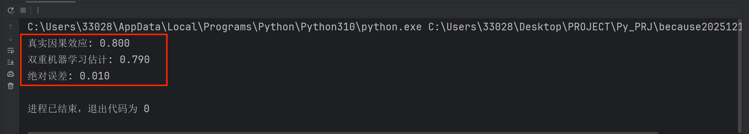

因果机器学习的实战：Uplift建模

在营销中，我们想知道：给用户发优惠券，到底能增加多少购买概率？

传统方法：对比发券组和未发券组的购买率。

问题：发券组本来购买意愿就高（选择偏差）。

Uplift建模：估计每个用户的个体处理效应。

对于本来就要买的用户：发券是浪费
对于不发就不买的用户：发券才有效

python 复制代码

# 简化的Uplift建模示例
import numpy as np  # 添加这行导入语句
import pandas as pd
from sklearn.model_selection import train_test_split
from sklearn.ensemble import RandomForestClassifier

# 模拟用户数据
np.random.seed(42)
n_users = 2000
user_features = np.random.normal(size=(n_users, 10))
# 模拟潜在结果：Y0(不发券), Y1(发券)
Y0 = (0.3*user_features[:,0] + 0.5*user_features[:,1] +
      np.random.normal(0, 0.2, n_users) > 0).astype(int)
Y1 = (0.8 + 0.3*user_features[:,0] + 0.5*user_features[:,1] +
      np.random.normal(0, 0.2, n_users) > 0).astype(int)

# 模拟发券策略（基于部分特征）
T = (0.4*user_features[:,0] + 0.6*user_features[:,2] +
     np.random.normal(0, 0.3, n_users) > 0).astype(int)

# 观测结果（只能看到一种情况）
Y_obs = np.where(T==1, Y1, Y0)

# 传统模型：预测发券后的购买概率
df = pd.DataFrame(user_features, columns=[f'X{i}' for i in range(10)])
df['T'] = T
df['Y'] = Y_obs

X_train, X_test, T_train, T_test, Y_train, Y_test = train_test_split(
    user_features, T, Y_obs, test_size=0.2, random_state=42)

# 传统模型
model_traditional = RandomForestClassifier()
model_traditional.fit(X_train, Y_train)
acc_traditional = model_traditional.score(X_test, Y_test)

# Uplift模型：分别预测发券和不发券的情况
X_treat = X_train[T_train==1]
Y_treat = Y_train[T_train==1]
X_control = X_train[T_train==0]
Y_control = Y_train[T_train==0]

model_treat = RandomForestClassifier()
model_control = RandomForestClassifier()
model_treat.fit(X_treat, Y_treat)
model_control.fit(X_control, Y_control)

# 估计Uplift
uplift_test = (model_treat.predict_proba(X_test)[:,1] -
               model_control.predict_proba(X_test)[:,1])

print(f"传统模型准确率: {acc_traditional:.3f}")
print(f"Uplift模型估计的个体处理效应范围: [{uplift_test.min():.3f}, {uplift_test.max():.3f}]")
print(f"高Uplift用户比例(>0.3): {(uplift_test > 0.3).mean():.1%}")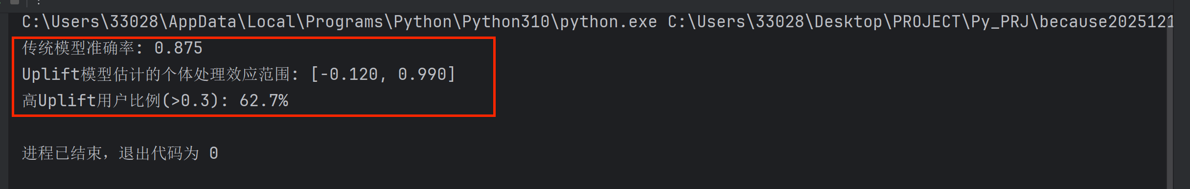

Uplift建模的价值：假设优惠券成本1元，转化利润10元。传统方法可能浪费大量预算在本来就会购买的用户身上，而Uplift建模可以精准定位那些"不发券不买，发券才买"的用户，将营销ROI提升2-5倍。

第二部分：可解释AI前沿------超越SHAP和LIME的"黑盒破解术"

SHAP和LIME的"中年危机"

SHAP（SHapley Additive exPlanations）和LIME（Local Interpretable Model-agnostic Explanations）无疑是可解释AI领域的明星。但它们正面临三大挑战：

局部性陷阱：每个预测单独解释，无法形成全局认知
特征工程依赖：解释的是特征重要性，而非人类可理解的概念
稳定性问题：相似的输入可能得到完全不同的解释

一个医疗诊断的典型案例：

python 复制代码

# 假设我们有一个AI诊断肺炎的模型
# 使用SHAP解释为什么某张X光片被诊断为肺炎
import shap

# 模拟模型预测和SHAP解释
def explain_with_shap(model, image):
    # SHAP会告诉你哪些像素重要
    explainer = shap.DeepExplainer(model, background_images)
    shap_values = explainer.shap_values(image)
    
    # 结果显示：右下肺叶的几个像素最重要
    # 但医生想问：为什么是这些像素？代表什么病理特征？
    
    return shap_values

医生真正关心的是：AI发现了什么医学特征？是毛玻璃影、实变还是胸腔积液？ 但SHAP只能回答：这些像素比较重要。

概念解释：让AI用人类的语言思考

概念解释的核心思想：不是解释特征重要性，而是解释模型学习了哪些人类可理解的概念。

Google Research提出的**TCAV（Testing with Concept Activation Vectors）**方法：

定义概念：如"条纹""圆形""毛玻璃影"
找到概念在模型内部表示的方向（概念激活向量）
测试模型预测对这个概念的敏感性

python 复制代码

# TCAV的简化思想演示
import numpy as np

# 假设模型内部有128维的表示
def model_internal_representation(image):
    # 实际中这是深度学习模型的某一层
    return np.random.normal(0, 1, 128)

# 定义"毛玻璃影"概念
def get_concept_vector(concept_name):
    # 实际中需要用有概念标注的数据训练
    concepts = {
        "毛玻璃影": np.array([0.8, -0.2, 0.3, ...]),  # 128维
        "实变": np.array([0.1, 0.9, -0.1, ...]),
        "胸腔积液": np.array([-0.3, 0.2, 0.7, ...]),
    }
    return concepts.get(concept_name, np.zeros(128))

# 计算概念敏感度
def concept_sensitivity(model_output, concept_vector):
    # 计算模型输出变化对概念方向的导数
    gradient = np.gradient(model_output, axis=0)  # 简化表示
    sensitivity = np.dot(gradient, concept_vector)
    return sensitivity

# 使用示例
image_rep = model_internal_representation(x_ray_image)
concept = get_concept_vector("毛玻璃影")
sensitivity = concept_sensitivity(pneumonia_probability, concept)
print(f"模型诊断对'毛玻璃影'概念的敏感度: {sensitivity:.3f}")

反事实解释：如果改变X，Y会怎样？

反事实解释回答的是：要达到不同的结果，输入应该如何最小程度地改变？

这在金融风控中特别有用：

用户问："为什么我的贷款被拒？"
传统回答："你的信用评分低，收入不足..."
反事实回答："如果你年收入增加5万元，或信用卡债务减少2万元，贷款就会被批准。"

python 复制代码

# 反事实解释的简化实现
import numpy as np
from sklearn.ensemble import RandomForestClassifier
from scipy.optimize import minimize

class CounterfactualExplainer:
    def __init__(self, model, feature_names, categorical_indices=[]):
        self.model = model
        self.feature_names = feature_names
        self.categorical_indices = categorical_indices
        
    def generate_counterfactual(self, x_original, desired_class, 
                                feature_weights=None, max_changes=3):
        """生成反事实解释"""
        n_features = len(x_original)
        if feature_weights is None:
            feature_weights = np.ones(n_features)
        
        def objective(x_candidate):
            # 距离成本
            distance_cost = np.sum(feature_weights * (x_candidate - x_original)**2)
            
            # 预测差异成本
            prob_original = self.model.predict_proba([x_original])[0]
            prob_candidate = self.model.predict_proba([x_candidate])[0]
            prediction_cost = (prob_original[desired_class] - 
                              prob_candidate[desired_class])**2
            
            # 稀疏性约束（限制改变的feature数量）
            changes = (np.abs(x_candidate - x_original) > 1e-3)
            sparsity_cost = max(0, changes.sum() - max_changes)**2
            
            return distance_cost + 10*prediction_cost + 5*sparsity_cost
        
        # 优化
        result = minimize(objective, x_original.copy(), 
                         bounds=[(0, 1) for _ in range(n_features)])
        
        return result.x
    
# 使用示例
np.random.seed(42)
n_samples = 1000
n_features = 10
X = np.random.rand(n_samples, n_features)
y = (X[:,0] + 0.5*X[:,1] - 0.3*X[:,2] > 0.5).astype(int)

model = RandomForestClassifier()
model.fit(X, y)

explainer = CounterfactualExplainer(model, feature_names=[f"F{i}" for i in range(n_features)])

# 用户被拒绝贷款（类别0）
user_features = np.random.rand(n_features)
prediction = model.predict([user_features])[0]

if prediction == 0:  # 被拒绝
    # 生成如何获得批准（类别1）的反事实
    counterfactual = explainer.generate_counterfactual(
        user_features, desired_class=1, max_changes=3)
    
    print("当前特征值:", user_features[:5])
    print("反事实特征值:", counterfactual[:5])
    print("需要改变的特征:")
    for i in range(n_features):
        if abs(counterfactual[i] - user_features[i]) > 0.1:  # 显著改变
            print(f"  {explainer.feature_names[i]}: {user_features[i]:.2f} -> {counterfactual[i]:.2f}")

临床决策支持的真实案例

梅奥诊所与MIT合作开发的可解释AI系统，用于败血症早期预警：

传统AI系统：提前4小时预测败血症风险，准确率85%
问题：医生不信任，因为不知道AI的推理过程
解决方案：加入概念解释
- 显示哪些生理指标异常（心率、血压、乳酸水平）
- 展示类似历史病例
- 提供反事实分析："如果乳酸水平降低，风险会如何变化"

结果：医生采纳率从30%提升到90%，每年多挽救数百条生命。

第三部分：AI for Science------当机器学习遇见自然法则

AlphaFold2：蛋白质结构预测的"登月时刻"

2020年，DeepMind的AlphaFold2在蛋白质结构预测竞赛CASP14中取得惊人成绩，平均误差约1.6Å（原子直径级别）。这不仅解决了生物学50年来的重大挑战，更展示了AI+科学的无限可能。

AlphaFold2的核心创新：

注意力机制的多序列对齐：从进化信息中提取结构线索
几何约束的端到端训练：直接预测原子坐标的3D结构
物理知识嵌入：结合化学键长、键角等先验知识

python 复制代码

# 简化的蛋白质结构预测思想
import numpy as np

def alphafold_simplified_idea(protein_sequence):
    """极度简化的AlphaFold思想演示"""
    # 1. 进化信息提取
    evolutionary_info = extract_evolutionary_info(protein_sequence)
    
    # 2. 多序列对齐（注意力机制）
    attention_weights = multi_sequence_attention(protein_sequence, evolutionary_info)
    
    # 3. 几何表示学习
    geometric_features = learn_geometric_representation(attention_weights)
    
    # 4. 物理约束优化
    structure = optimize_with_physical_constraints(geometric_features)
    
    return structure

# AlphaFold2的核心：从序列到结构的端到端学习
def e2e_protein_folding(sequence):
    """端到端蛋白质折叠的简化演示"""
    # 实际AlphaFold2有复杂的transformer架构
    # 这里只展示思想
    
    # 编码器：提取特征
    residue_features = transformer_encoder(sequence)
    
    # 结构模块：预测3D坐标
    # 使用SE(3)等变网络，保证旋转平移不变性
    coordinates = structure_module(residue_features)
    
    # 迭代优化
    for _ in range(3):  # AlphaFold2有3次迭代
        confidence_scores = confidence_module(coordinates, residue_features)
        coordinates = refinement_module(coordinates, residue_features, confidence_scores)
    
    return coordinates, confidence_scores

AlphaFold2的影响远不止蛋白质：

药物发现：快速筛选靶点
疾病研究：理解突变如何影响结构
合成生物学：设计全新蛋白质

气候建模：从物理方程到数据驱动的融合

传统气候模型基于物理方程，计算代价高昂。AI气候模型通过学习观测数据，可以快几个数量级地预测气候变化。

python 复制代码

# 气候建模的AI方法演示
import numpy as np
from sklearn.ensemble import RandomForestRegressor
from sklearn.neural_network import MLPRegressor

class HybridClimateModel:
    """混合气候模型：结合物理知识和机器学习"""
    def __init__(self, physical_constraints=True):
        self.physical_constraints = physical_constraints
        
    def train(self, historical_data, future_scenarios):
        """训练混合模型"""
        # 历史数据：温度、CO2浓度、太阳辐射等
        X_train, y_train = self.preprocess_data(historical_data)
        
        if self.physical_constraints:
            # 加入物理约束的机器学习
            self.model = self.physically_constrained_ml(X_train, y_train)
        else:
            # 纯数据驱动
            self.model = MLPRegressor(hidden_layer_sizes=(100, 50))
            self.model.fit(X_train, y_train)
    
    def physically_constrained_ml(self, X, y):
        """物理约束的机器学习"""
        # 1. 能量守恒约束
        def energy_constraint(predictions):
            # 简化：全球能量平衡
            return np.abs(predictions.sum() - X[:,0].sum())  # 粗略约束
        
        # 2. 使用可解释模型
        model = RandomForestRegressor(n_estimators=100)
        model.fit(X, y)
        
        # 3. 后处理调整以满足物理约束
        return model
    
    def predict(self, current_conditions, years_ahead):
        """预测未来气候"""
        predictions = []
        current = current_conditions
        
        for year in range(years_ahead):
            # 使用模型预测下一步
            next_step = self.model.predict([current])[0]
            
            # 应用物理约束修正
            if self.physical_constraints:
                next_step = self.apply_physical_constraints(current, next_step)
            
            predictions.append(next_step)
            current = next_step  # 自回归预测
        
        return np.array(predictions)

AI气候模型的优势：

速度：传统模型需要超级计算机运行数周，AI模型只需几小时
不确定性量化：可以估计预测的置信区间
极端事件预测：更好地预测热浪、洪水等极端天气

材料发现：加速新材料研发10倍

传统材料研发靠"试错"，发现一种新材料平均需要10-20年。AI可以将这个过程缩短到1-2年。

python 复制代码

# 材料发现的AI工作流
class MaterialsDiscoveryAI:
    def __init__(self):
        self.property_predictor = None
        self.generator = None
        
    def workflow(self):
        """AI材料发现的工作流"""
        steps = {
            "1. 数据收集": "从文献、实验中收集材料数据",
            "2. 特征工程": "提取晶体结构、化学成分等特征",
            "3. 性质预测": "用机器学习预测材料的导电性、强度等",
            "4. 生成设计": "用生成模型设计新材料结构",
            "5. 实验验证": "合成最有前途的候选材料",
            "6. 反馈循环": "用实验结果改进AI模型"
        }
        return steps
    
    def discover_superconductor(self, target_temperature=150):  # 150K超导体
        """发现高温超导体的简化演示"""
        # 1. 搜索材料空间
        candidate_materials = self.search_material_space(
            elements=["Cu", "Ba", "Y", "O"],  # 类似YBCO的元素
            structure_types=["perovskite", "layered"]
        )
        
        # 2. 预测超导温度
        predictions = []
        for material in candidate_materials:
            tc_pred = self.predict_tc(material)  # 预测临界温度
            confidence = self.prediction_confidence(material)
            predictions.append((material, tc_pred, confidence))
        
        # 3. 选择最有希望的候选
        predictions.sort(key=lambda x: x[1], reverse=True)
        best_candidates = predictions[:10]  # 前10个
        
        # 4. 考虑合成可行性
        feasible_candidates = self.filter_by_synthesis_feasibility(best_candidates)
        
        return feasible_candidates

实际成果：伯克利实验室的"材料项目"已发现数千种有前途的新材料，其中几十种已实验验证。

第四部分：决策智能------当优化遇见机器学习

传统运筹学的局限

运筹学研究优化问题：资源分配、路径规划、库存管理。但它有两大局限：

精确模型依赖：需要精确知道所有参数
静态优化：一旦环境变化，解可能不再最优

强化学习+运筹学：自适应优化

强化学习通过试错学习最优策略，正好弥补运筹学的不足。

动态定价案例：航空公司如何实时调整票价？

python 复制代码

import numpy as np
import matplotlib
import matplotlib.pyplot as plt
# 配置中文字体（根据您的系统选择合适的方法）

# 方法1：使用系统自带的中文字体（Windows系统）
plt.rcParams['font.sans-serif'] = ['SimHei']  # 用来正常显示中文标签
plt.rcParams['axes.unicode_minus'] = False  # 用来正常显示负号


class DynamicPricingAgent:
    """动态定价智能体"""

    def __init__(self, n_price_levels=10):
        self.n_price_levels = n_price_levels
        self.demand_bins = 5
        self.competition_bins = 5
        self.n_states = self.demand_bins * self.competition_bins
        # 修正：Q表应该是状态数×动作数
        self.q_table = np.zeros((self.n_states, n_price_levels))
        self.learning_rate = 0.1
        self.discount_factor = 0.9
        self.epsilon = 0.1  # 探索率

    def state_representation(self, market_conditions):
        """将市场状况编码为状态"""
        # 简化：基于需求水平和竞争价格
        demand_level = self.discretize(market_conditions['demand'], self.demand_bins)
        competition_price = self.discretize(market_conditions['competition_price'], self.competition_bins)
        return (demand_level, competition_price)

    def discretize(self, value, n_bins):
        """连续值离散化"""
        # 确保值在[0, 1]范围内
        value = max(0, min(1, value))
        return min(int(value * n_bins), n_bins - 1)

    def state_to_index(self, state):
        """将二维状态转换为一维索引"""
        demand_idx, competition_idx = state
        return demand_idx * self.competition_bins + competition_idx

    def choose_price(self, state, current_price):
        """选择价格动作"""
        if np.random.random() < self.epsilon:
            # 探索：随机选择价格
            return np.random.randint(0, self.n_price_levels)
        else:
            # 利用：选择Q值最高的价格
            state_idx = self.state_to_index(state)
            return np.argmax(self.q_table[state_idx])

    def update(self, state, action, reward, next_state):
        """更新Q表"""
        state_idx = self.state_to_index(state)
        next_state_idx = self.state_to_index(next_state)

        # Q-learning更新公式
        current_q = self.q_table[state_idx, action]
        max_future_q = np.max(self.q_table[next_state_idx])
        new_q = current_q + self.learning_rate * (
                reward + self.discount_factor * max_future_q - current_q
        )
        self.q_table[state_idx, action] = new_q

    def simulate_market(self, days=100):
        """模拟市场环境"""
        prices = []
        revenues = []
        # 初始状态：中等需求和中等竞争价格
        current_state = (2, 2)
        current_price_idx = 5  # 中间价格

        for day in range(days):
            # 市场条件变化
            market_conditions = {
                'demand': np.clip(np.random.normal(0.5, 0.1), 0, 1),  # 限制在[0,1]
                'competition_price': np.clip(np.random.normal(0.6, 0.15), 0, 1)  # 限制在[0,1]
            }

            # 当前状态
            state = self.state_representation(market_conditions)

            # 选择价格动作
            price_action = self.choose_price(state, current_price_idx)

            # 价格索引转实际价格
            price = 100 + price_action * 20  # 假设价格范围100-280

            # 模拟需求响应（价格弹性）
            base_demand = 100 * market_conditions['demand']
            price_elasticity = -1.5
            demand = base_demand * (price / 200) ** price_elasticity

            # 收益
            revenue = price * demand

            # 奖励（考虑市场份额）
            competition_price = market_conditions['competition_price'] * 200
            competition_ratio = price / competition_price if competition_price > 0 else 2.0
            if competition_ratio < 1.1:  # 价格不超过竞争对手10%
                market_share = 0.5
            else:
                market_share = 0.2

            reward = revenue * market_share

            # 下一状态
            next_market_conditions = {
                'demand': np.clip(
                    market_conditions['demand'] + np.random.normal(0, 0.05), 0, 1
                ),
                'competition_price': np.clip(
                    market_conditions['competition_price'] + np.random.normal(0, 0.03), 0, 1
                )
            }
            next_state = self.state_representation(next_market_conditions)

            # 更新Q表
            self.update(state, price_action, reward, next_state)

            # 更新当前价格和状态
            current_price_idx = price_action
            current_state = state

            prices.append(price)
            revenues.append(revenue)

            # 衰减探索率
            self.epsilon *= 0.995

        return prices, revenues


# 运行模拟
agent = DynamicPricingAgent()
prices, revenues = agent.simulate_market(days=200)

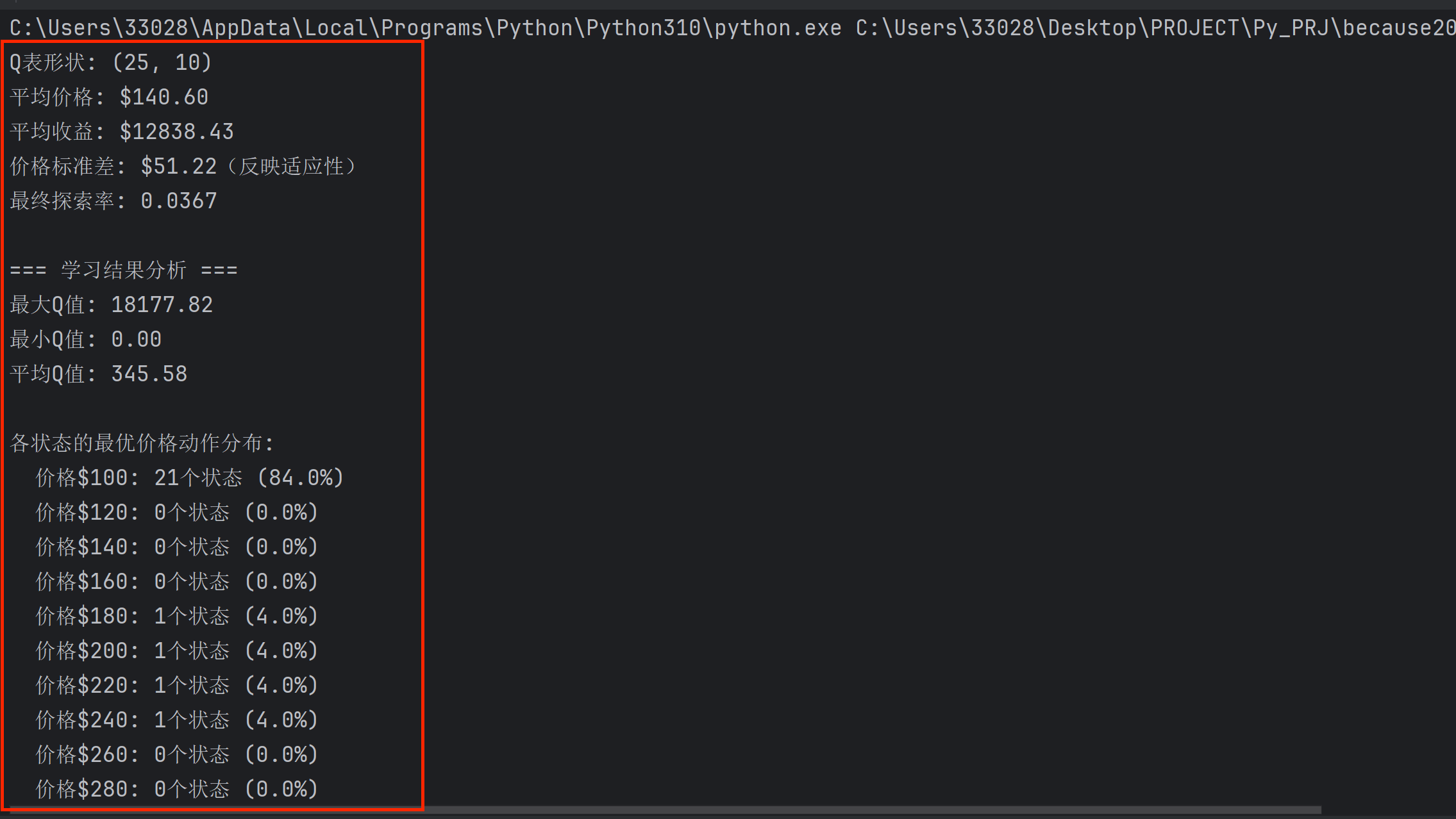
print(f"Q表形状: {agent.q_table.shape}")
print(f"平均价格: ${np.mean(prices):.2f}")
print(f"平均收益: ${np.mean(revenues):.2f}")
print(f"价格标准差: ${np.std(prices):.2f}（反映适应性）")
print(f"最终探索率: {agent.epsilon:.4f}")

# 可视化学习过程
import matplotlib.pyplot as plt

fig, axes = plt.subplots(2, 2, figsize=(12, 10))

# 价格随时间变化
axes[0, 0].plot(prices)
axes[0, 0].set_xlabel('天数')
axes[0, 0].set_ylabel('价格 ($)')
axes[0, 0].set_title('价格随时间变化')
axes[0, 0].grid(True)

# 收益随时间变化
axes[0, 1].plot(revenues)
axes[0, 1].set_xlabel('天数')
axes[0, 1].set_ylabel('收益 ($)')
axes[0, 1].set_title('收益随时间变化')
axes[0, 1].grid(True)

# 价格分布直方图
axes[1, 0].hist(prices, bins=20, edgecolor='black', alpha=0.7)
axes[1, 0].set_xlabel('价格 ($)')
axes[1, 0].set_ylabel('频次')
axes[1, 0].set_title('价格分布')
axes[1, 0].grid(True)

# Q表热力图
im = axes[1, 1].imshow(agent.q_table, aspect='auto', cmap='hot')
axes[1, 1].set_xlabel('价格动作')
axes[1, 1].set_ylabel('状态索引')
axes[1, 1].set_title('Q表热力图')
plt.colorbar(im, ax=axes[1, 1], label='Q值')

plt.tight_layout()
plt.show()

# 分析学习结果
print("\n=== 学习结果分析 ===")
print(f"最大Q值: {np.max(agent.q_table):.2f}")
print(f"最小Q值: {np.min(agent.q_table):.2f}")
print(f"平均Q值: {np.mean(agent.q_table):.2f}")

# 找到最优策略
optimal_policy = np.argmax(agent.q_table, axis=1)
print(f"\n各状态的最优价格动作分布:")
for action in range(agent.n_price_levels):
    count = np.sum(optimal_policy == action)
    price = 100 + action * 20
    print(f"  价格${price}: {count}个状态 ({count / len(optimal_policy):.1%})")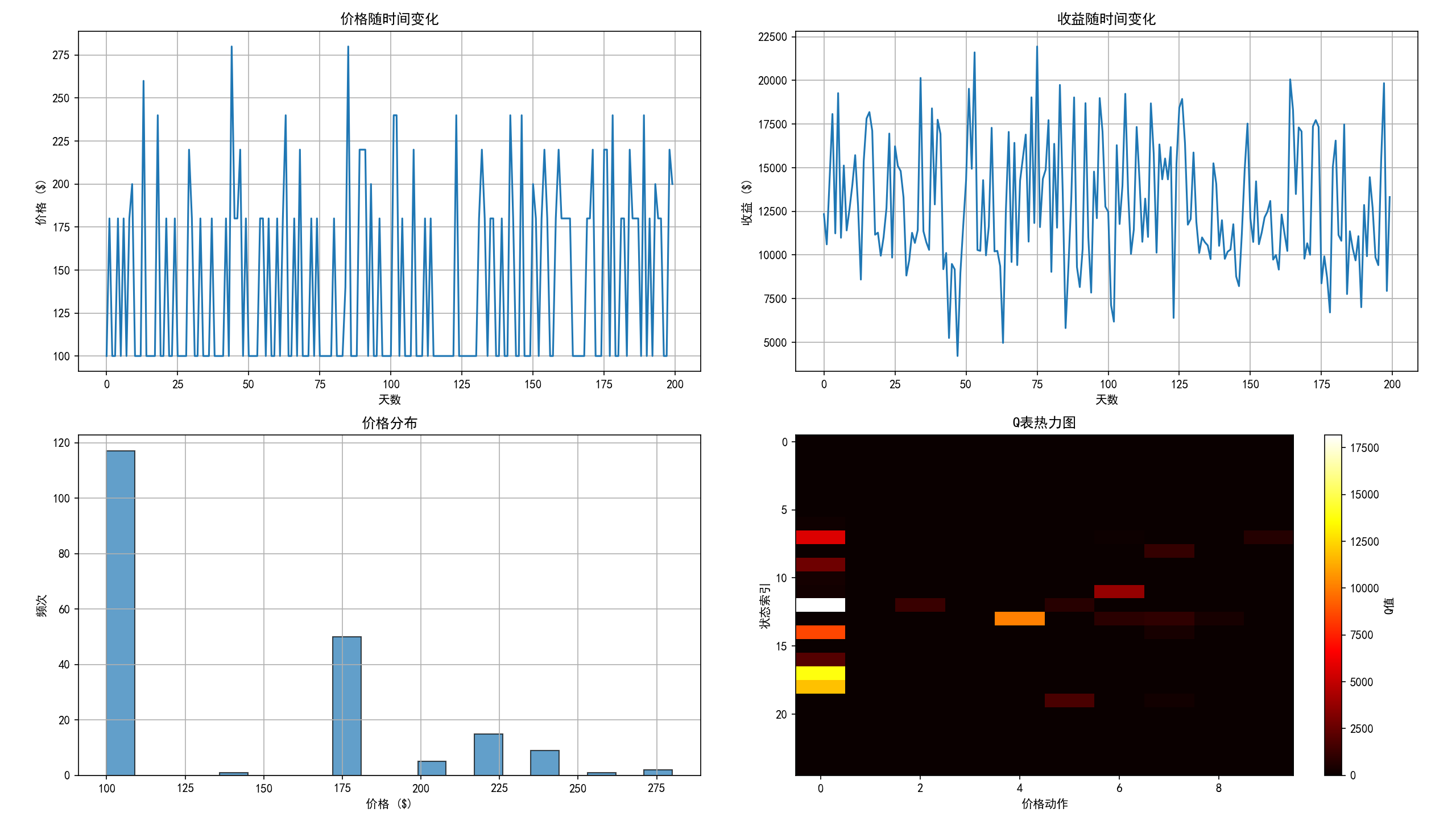

决策智能的实际应用：

物流优化：UPS的ORION系统结合运筹学和机器学习，每年节省1亿英里路程
能源管理：谷歌数据中心使用AI优化冷却，能效提升40%
金融投资：BlackRock的Aladdin平台管理21万亿美元资产

结语：从预测到理解，从优化到创造

我们走过了因果机器学习的严谨推理、可解释AI的透明决策、科学发现的跨界融合、决策智能的动态优化。这不仅仅是技术的演进，更是机器学习范式的根本转变。

三个关键转变

从相关性到因果性：不再满足于"是什么"，而要追问"为什么"
从黑盒到玻璃盒：AI的决策过程需要透明、可解释、可信任
从数据驱动到知识融合：结合领域知识、物理定律、人类直觉