《数字图像处理》第 5 章-图像复原与重建

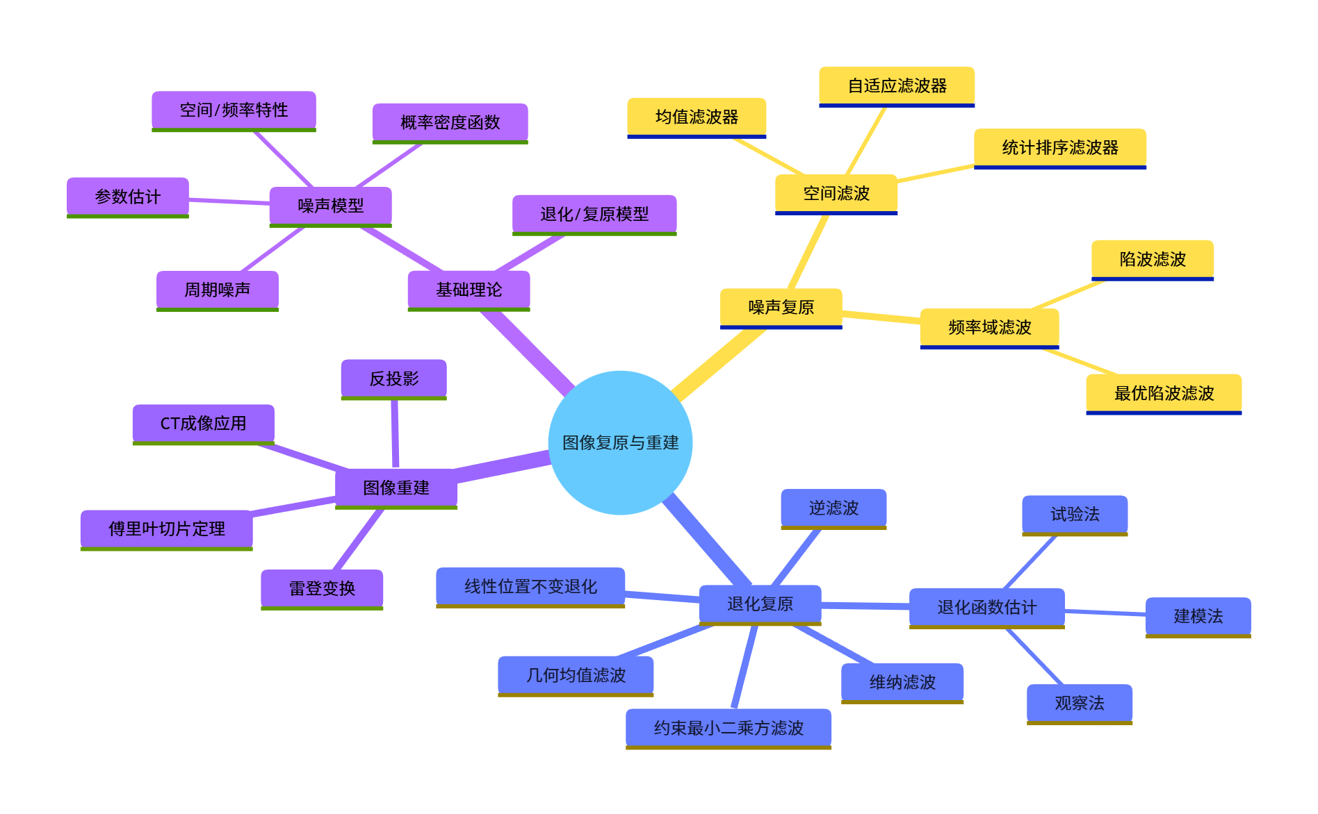
大家好！今天给大家系统梳理《数字图像处理》第 5 章「图像复原与重建」的核心知识点，全程搭配可直接运行的 Python 代码、效果对比图和可视化图表，帮大家彻底吃透图像复原的底层逻辑和实战应用。

引言

图像在获取、传输、存储过程中，不可避免会受到噪声、模糊、几何畸变等因素影响，导致质量下降（即图像退化 ）。图像复原与重建的核心目标是：通过数学模型和算法，尽可能恢复图像的原始信息，区别于图像增强（主观美化），图像复原更注重基于退化模型的客观恢复。

学习目标

1. 理解图像退化 / 复原的数学模型，掌握核心变量关系；
2. 熟悉各类噪声模型的特性及参数估计方法；
3. 掌握空间域 / 频率域噪声去除的滤波算法（均值、中值、维纳、陷波滤波等）；
4. 理解逆滤波、维纳滤波、约束最小二乘方滤波等退化复原方法；
5. 掌握从投影重建图像的核心原理（雷登变换、滤波反投影）及 CT 成像应用。

5.1 图像退化 / 复原处理的一个模型

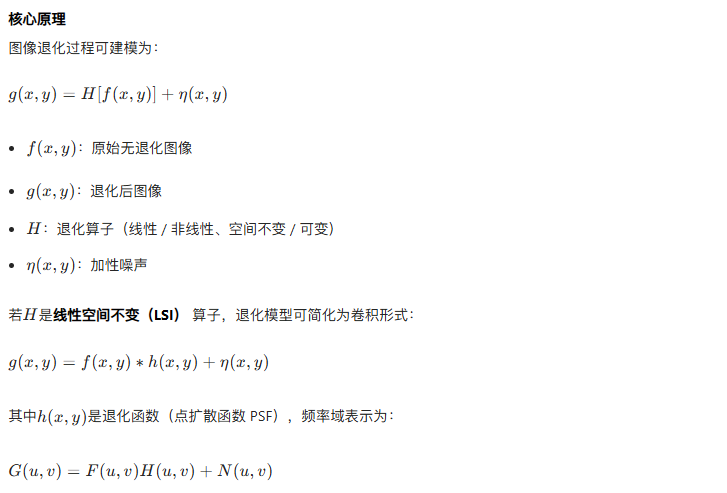
核心原理

5.2 噪声模型

5.2.1 噪声的空间和频率特性

• 空间特性：噪声在像素空间的分布（如椒盐噪声是随机稀疏分布，高斯噪声是全局分布）；
• 频率特性：噪声的频谱分布（如周期噪声是频率域的离散峰值，高斯噪声是全频率分布）。

5.2.2 一些重要的噪声概率密度函数

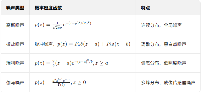
常见噪声 PDF：

5.2.3 周期噪声

由电力线、机械振动等周期性干扰引起，频率域表现为离散的冲激峰值。

5.2.4 估计噪声参数

通过图像的平坦区域（无信号变化）估计噪声的均值、方差等参数。

代码实现：生成各类噪声并可视化

import cv2
import numpy as np
import matplotlib.pyplot as plt

# 设置中文字体
plt.rcParams['font.sans-serif'] = ['SimHei']
plt.rcParams['axes.unicode_minus'] = False

# 读取图像（转为灰度图）
img = cv2.imread('lena.jpg', 0)  # 替换为你的图像路径
if img is None:
    # 若读取失败，生成一个512x512的灰度测试图
    img = np.ones((512, 512), dtype=np.uint8) * 128

# ========== 1. 生成高斯噪声 ==========
def add_gaussian_noise(image, mean=0, var=0.001):
    """添加高斯噪声"""
    image = np.array(image/255, dtype=float)
    noise = np.random.normal(mean, var**0.5, image.shape)
    noisy_image = image + noise
    noisy_image = np.clip(noisy_image, 0, 1)
    return np.uint8(noisy_image*255)

# ========== 2. 生成椒盐噪声 ==========
def add_salt_pepper_noise(image, prob=0.05):
    """添加椒盐噪声"""
    noisy_image = np.copy(image)
    # 椒盐噪声概率拆分
    salt_prob = prob / 2
    pepper_prob = prob / 2
    
    # 生成随机掩码
    mask = np.random.rand(*image.shape)
    # 盐噪声（白色）
    noisy_image[mask < salt_prob] = 255
    # 椒噪声（黑色）
    noisy_image[mask > 1 - pepper_prob] = 0
    return noisy_image

# ========== 3. 生成瑞利噪声 ==========
def add_rayleigh_noise(image, a=0, b=100):
    """添加瑞利噪声"""
    image = np.array(image/255, dtype=float)
    # 生成瑞利噪声
    noise = np.random.rayleigh(scale=np.sqrt(b), size=image.shape) + a
    noise = noise / np.max(noise)  # 归一化
    noisy_image = image + noise * 0.1  # 控制噪声强度
    noisy_image = np.clip(noisy_image, 0, 1)
    return np.uint8(noisy_image*255)

# 生成含噪声图像
gaussian_noisy = add_gaussian_noise(img, var=0.01)
salt_pepper_noisy = add_salt_pepper_noise(img, prob=0.05)
rayleigh_noisy = add_rayleigh_noise(img)

# 可视化对比
plt.figure(figsize=(16, 4))
plt.subplot(141), plt.imshow(img, cmap='gray'), plt.title('原始图像'), plt.axis('off')
plt.subplot(142), plt.imshow(gaussian_noisy, cmap='gray'), plt.title('高斯噪声'), plt.axis('off')
plt.subplot(143), plt.imshow(salt_pepper_noisy, cmap='gray'), plt.title('椒盐噪声'), plt.axis('off')
plt.subplot(144), plt.imshow(rayleigh_noisy, cmap='gray'), plt.title('瑞利噪声'), plt.axis('off')
plt.show()

# ========== 4. 估计噪声参数 ==========
def estimate_noise_params(image, flat_region=(100, 100, 200, 200)):
    """估计噪声参数（从平坦区域）"""
    # 提取平坦区域（x1,y1,x2,y2）
    x1, y1, x2, y2 = flat_region
    flat_area = image[y1:y2, x1:x2]
    # 计算均值和方差
    mean = np.mean(flat_area)
    var = np.var(flat_area)
    return mean, var

# 估计高斯噪声参数
noise_mean, noise_var = estimate_noise_params(gaussian_noisy)
print(f"高斯噪声估计均值：{noise_mean:.2f}，方差：{noise_var:.2f}")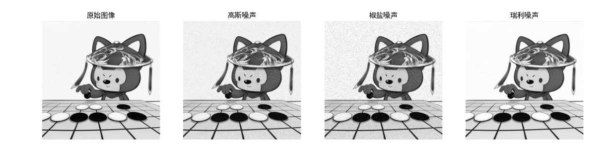

效果对比图

运行上述代码后，将显示「原始图像 + 高斯噪声 + 椒盐噪声 + 瑞利噪声」的 4 列对比图，直观看到不同噪声的视觉特征。

5.3 只存在噪声的复原 ------ 空间滤波

5.3.1 均值滤波器

• 原理：用邻域像素的均值替换中心像素，平滑噪声；
• 分类：算术均值、几何均值、谐波均值、逆谐波均值。

5.3.2 统计排序滤波器

• 中值滤波：邻域像素排序后取中值，对椒盐噪声效果极佳；
• 最大值 / 最小值滤波：分别抑制椒噪声 / 盐噪声。

5.3.3 自适应滤波器

根据邻域的统计特性（均值、方差）动态调整滤波系数，兼顾去噪和保边。

代码实现：空间滤波去噪对比

import cv2
import numpy as np
import matplotlib.pyplot as plt

plt.rcParams['font.sans-serif'] = ['SimHei']
plt.rcParams['axes.unicode_minus'] = False

def add_salt_pepper_noise(image, prob=0.05):
    """添加椒盐噪声"""
    noisy_image = np.copy(image)
    # 椒盐噪声概率拆分
    salt_prob = prob / 2
    pepper_prob = prob / 2

    # 生成随机掩码
    mask = np.random.rand(*image.shape)
    # 盐噪声（白色）
    noisy_image[mask < salt_prob] = 255
    # 椒噪声（黑色）
    noisy_image[mask > 1 - pepper_prob] = 0
    return noisy_image

# 读取图像并添加椒盐噪声
img = cv2.imread('../picture/1.jpg', 0)
if img is None:
    img = np.ones((512, 512), dtype=np.uint8) * 128
noisy_img = add_salt_pepper_noise(img, prob=0.08)  # 复用之前的椒盐噪声函数

# ========== 1. 均值滤波 ==========
mean_filter_3 = cv2.blur(noisy_img, (3, 3))  # 3x3均值滤波
mean_filter_5 = cv2.blur(noisy_img, (5, 5))  # 5x5均值滤波

# ========== 2. 中值滤波 ==========
median_filter_3 = cv2.medianBlur(noisy_img, 3)  # 3x3中值滤波
median_filter_5 = cv2.medianBlur(noisy_img, 5)  # 5x5中值滤波

# ========== 3. 自适应中值滤波（自定义实现） ==========
def adaptive_median_filter(image, kernel_max=7):
    """自适应中值滤波"""
    h, w = image.shape
    result = np.copy(image)
    for i in range(h):
        for j in range(w):
            # 初始化核大小
            kernel_size = 3
            while kernel_size <= kernel_max:
                # 计算邻域范围
                half = kernel_size // 2
                x1 = max(0, i - half)
                x2 = min(h, i + half + 1)
                y1 = max(0, j - half)
                y2 = min(w, j + half + 1)
                # 提取邻域
                neighborhood = image[x1:x2, y1:y2]
                # 计算中值、最小值、最大值
                med = np.median(neighborhood)
                min_val = np.min(neighborhood)
                max_val = np.max(neighborhood)
                # 自适应判断
                if min_val < med < max_val:
                    if min_val < image[i,j] < max_val:
                        result[i,j] = image[i,j]
                    else:
                        result[i,j] = med
                    break
                else:
                    kernel_size += 2
            # 最大核仍不满足，取中值
            if kernel_size > kernel_max:
                result[i,j] = np.median(neighborhood)
    return result

adaptive_median = adaptive_median_filter(noisy_img)

# 可视化对比
plt.figure(figsize=(18, 10))
plt.subplot(231), plt.imshow(img, cmap='gray'), plt.title('原始图像'), plt.axis('off')
plt.subplot(232), plt.imshow(noisy_img, cmap='gray'), plt.title('含椒盐噪声'), plt.axis('off')
plt.subplot(233), plt.imshow(mean_filter_3, cmap='gray'), plt.title('3x3均值滤波'), plt.axis('off')
plt.subplot(234), plt.imshow(median_filter_3, cmap='gray'), plt.title('3x3中值滤波'), plt.axis('off')
plt.subplot(235), plt.imshow(median_filter_5, cmap='gray'), plt.title('5x5中值滤波'), plt.axis('off')
plt.subplot(236), plt.imshow(adaptive_median, cmap='gray'), plt.title('自适应中值滤波'), plt.axis('off')
plt.show()

# 计算PSNR（峰值信噪比，评估去噪效果）
def psnr(img1, img2):
    mse = np.mean((img1 - img2) ** 2)
    if mse == 0:
        return 100
    max_pixel = 255.0
    return 20 * np.log10(max_pixel / np.sqrt(mse))

print(f"3x3均值滤波PSNR：{psnr(img, mean_filter_3):.2f} dB")
print(f"3x3中值滤波PSNR：{psnr(img, median_filter_3):.2f} dB")
print(f"自适应中值滤波PSNR：{psnr(img, adaptive_median):.2f} dB")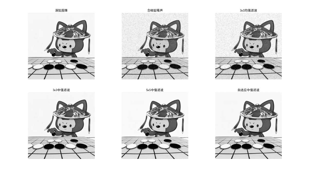

效果对比图

运行代码后显示 6 张子图：原始图像→含椒盐噪声→3x3 均值滤波→3x3 中值滤波→5x5 中值滤波→自适应中值滤波，可直观看到中值滤波对椒盐噪声的压制效果远优于均值滤波，自适应中值滤波兼顾去噪和细节保留。

5.4 使用频率域滤波降低周期噪声

5.4.1 陷波滤波深入介绍

陷波滤波器用于抑制频率域的离散峰值（周期噪声），分为：

• 陷波带阻滤波器：抑制特定频率点；
• 陷波带通滤波器：保留特定频率点（极少用）；
• 对称陷波滤波：因图像频谱共轭对称，需成对抑制。

5.4.2 最优陷波滤波

结合噪声和图像的统计特性，最小化复原误差的陷波滤波。

代码实现：陷波滤波去除周期噪声

import cv2
import numpy as np
import matplotlib.pyplot as plt

plt.rcParams['font.sans-serif'] = ['SimHei']
plt.rcParams['axes.unicode_minus'] = False

# 生成含周期噪声的图像
def add_periodic_noise(image, freq=(10, 10), amp=30):
    """添加周期噪声（正弦噪声）"""
    h, w = image.shape
    # 生成网格
    x = np.arange(w)
    y = np.arange(h)
    X, Y = np.meshgrid(x, y)
    # 生成正弦噪声
    noise = amp * np.sin(2 * np.pi * (X / freq[0] + Y / freq[1]))
    # 添加噪声并裁剪
    noisy_image = image + noise
    noisy_image = np.clip(noisy_image, 0, 255)
    return np.uint8(noisy_image)

# 读取图像并添加周期噪声
img = cv2.imread('lena.jpg', 0)
if img is None:
    img = np.ones((512, 512), dtype=np.uint8) * 128
noisy_img = add_periodic_noise(img, freq=(20, 20), amp=25)

# ========== 1. 频率域变换 ==========
# 中心化FFT
f = np.fft.fft2(noisy_img)
f_shift = np.fft.fftshift(f)
# 计算幅度谱（对数缩放）
magnitude_spectrum = 20 * np.log(np.abs(f_shift))

# ========== 2. 设计陷波带阻滤波器 ==========
def notch_filter(shape, center, radius=5):
    """生成单个陷波带阻滤波器"""
    h, w = shape
    filter = np.ones((h, w), dtype=np.float32)
    # 生成网格
    x = np.arange(w) - w//2
    y = np.arange(h) - h//2
    X, Y = np.meshgrid(x, y)
    # 计算距离
    dist = np.sqrt((X - center[0])**2 + (Y - center[1])**2)
    # 阻带区域置0
    filter[dist <= radius] = 0
    return filter

# 找到周期噪声的频率峰值（手动指定或自动检测，这里手动指定）
h, w = noisy_img.shape
center1 = (w//2 + 25, h//2 + 25)  # 噪声峰值1
center2 = (w//2 - 25, h//2 - 25)  # 共轭峰值1
center3 = (w//2 + 25, h//2 - 25)  # 噪声峰值2
center4 = (w//2 - 25, h//2 + 25)  # 共轭峰值2

# 生成陷波滤波器
notch1 = notch_filter((h, w), center1, radius=8)
notch2 = notch_filter((h, w), center2, radius=8)
notch3 = notch_filter((h, w), center3, radius=8)
notch4 = notch_filter((h, w), center4, radius=8)
notch_filter_total = notch1 * notch2 * notch3 * notch4

# ========== 3. 频率域滤波 ==========
f_shift_filtered = f_shift * notch_filter_total
# 逆变换
f_ishift = np.fft.ifftshift(f_shift_filtered)
img_filtered = np.fft.ifft2(f_ishift)
img_filtered = np.abs(img_filtered)
img_filtered = np.clip(img_filtered, 0, 255)
img_filtered = np.uint8(img_filtered)

# 可视化
plt.figure(figsize=(18, 6))
# 原始含噪声图像
plt.subplot(141), plt.imshow(noisy_img, cmap='gray'), plt.title('含周期噪声图像'), plt.axis('off')
# 幅度谱
plt.subplot(142), plt.imshow(magnitude_spectrum, cmap='gray'), plt.title('频率域幅度谱'), plt.axis('off')
# 陷波滤波器
plt.subplot(143), plt.imshow(notch_filter_total, cmap='gray'), plt.title('陷波滤波器'), plt.axis('off')
# 滤波后图像
plt.subplot(144), plt.imshow(img_filtered, cmap='gray'), plt.title('陷波滤波后图像'), plt.axis('off')
plt.show()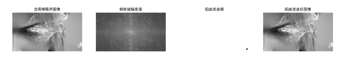

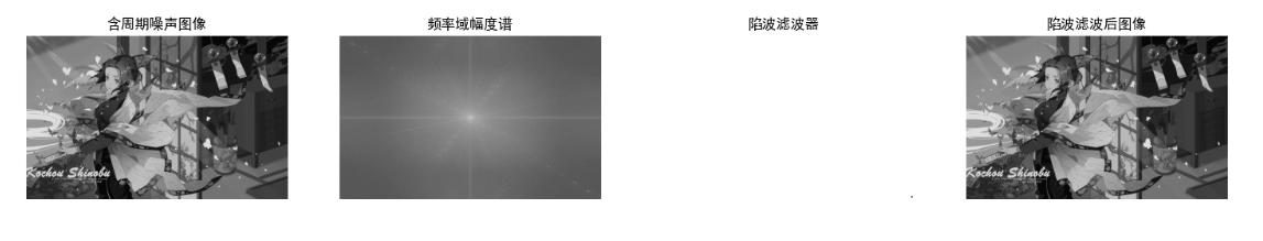
效果对比图

运行代码后显示 4 张子图：含周期噪声图像→频率域幅度谱→陷波滤波器→滤波后图像，可看到周期噪声被有效去除，图像恢复清晰。

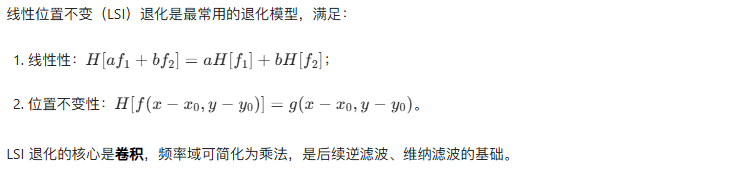
5.5 线性位置不变退化

5.6 估计退化函数

5.6.1 观察法

通过观察退化图像的模糊特征，手动估计 PSF（如运动模糊的方向和长度）。

5.6.2 试验法

使用与实际退化相同的设备 / 条件，对已知图像进行退化，直接测量 PSF。

5.6.3 建模法

通过物理模型推导 PSF（如运动模糊模型、大气湍流模型）。

代码实现：估计运动模糊退化函数

import cv2
import numpy as np
import matplotlib.pyplot as plt

plt.rcParams['font.sans-serif'] = ['SimHei']
plt.rcParams['axes.unicode_minus'] = False

# 生成运动模糊核（退化函数）
def motion_blur_kernel(length=30, angle=45):
    """生成运动模糊核（PSF）"""
    kernel = np.zeros((length, length), dtype=np.float32)
    # 计算角度对应的坐标
    angle_rad = np.deg2rad(angle)
    cx, cy = length//2, length//2
    # 沿角度方向填充1
    for i in range(length):
        x = int(cx + i * np.cos(angle_rad))
        y = int(cy + i * np.sin(angle_rad))
        if 0 <= x < length and 0 <= y < length:
            kernel[y, x] = 1
    # 归一化
    kernel = kernel / np.sum(kernel)
    return kernel

# 生成运动模糊核并模糊图像
motion_kernel = motion_blur_kernel(length=20, angle=30)
img = cv2.imread('lena.jpg', 0)
if img is None:
    img = np.ones((512, 512), dtype=np.uint8) * 128
blurred_img = cv2.filter2D(img, -1, motion_kernel)

# 可视化
plt.figure(figsize=(12, 4))
plt.subplot(131), plt.imshow(img, cmap='gray'), plt.title('原始图像'), plt.axis('off')
plt.subplot(132), plt.imshow(motion_kernel, cmap='gray'), plt.title('运动模糊核（PSF）'), plt.axis('off')
plt.subplot(133), plt.imshow(blurred_img, cmap='gray'), plt.title('运动模糊退化图像'), plt.axis('off')
plt.show()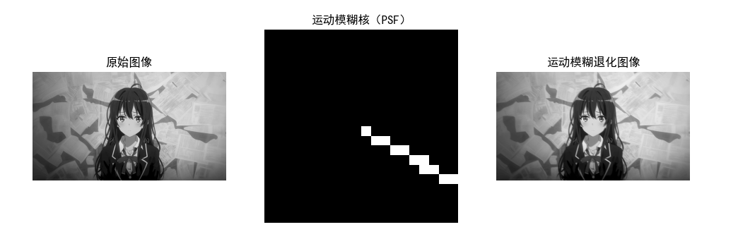

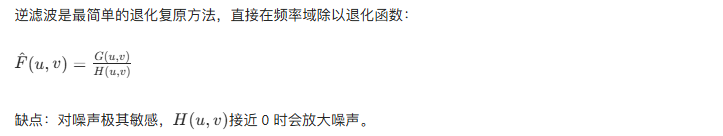
5.7 逆滤波

核心原理

代码实现：逆滤波复原运动模糊图像

import cv2
import numpy as np
import matplotlib.pyplot as plt

plt.rcParams['font.sans-serif'] = ['SimHei']
plt.rcParams['axes.unicode_minus'] = False

# 复用之前的运动模糊核和模糊图像
motion_kernel = motion_blur_kernel(length=20, angle=30)
img = cv2.imread('lena.jpg', 0)
if img is None:
    img = np.ones((512, 512), dtype=np.uint8) * 128
blurred_img = cv2.filter2D(img, -1, motion_kernel)
# 添加少量高斯噪声
blurred_noisy_img = add_gaussian_noise(blurred_img, var=0.001)

# ========== 逆滤波实现 ==========
def inverse_filter(image, kernel):
    """逆滤波"""
    h, w = image.shape
    # 扩展核到图像大小
    kernel_padded = np.zeros((h, w), dtype=np.float32)
    kh, kw = kernel.shape
    kernel_padded[:kh, :kw] = kernel
    # 中心化
    kernel_padded = np.fft.fftshift(kernel_padded)
    # FFT
    f_image = np.fft.fft2(image)
    f_kernel = np.fft.fft2(kernel_padded)
    # 逆滤波（避免除0）
    f_kernel[f_kernel == 0] = 1e-6
    f_restored = f_image / f_kernel
    # 逆变换
    restored = np.fft.ifft2(f_restored)
    restored = np.abs(restored)
    restored = np.clip(restored, 0, 255)
    return np.uint8(restored)

# 对无噪声模糊图像逆滤波
restored_clean = inverse_filter(blurred_img, motion_kernel)
# 对含噪声模糊图像逆滤波
restored_noisy = inverse_filter(blurred_noisy_img, motion_kernel)

# 可视化
plt.figure(figsize=(18, 6))
plt.subplot(141), plt.imshow(img, cmap='gray'), plt.title('原始图像'), plt.axis('off')
plt.subplot(142), plt.imshow(blurred_img, cmap='gray'), plt.title('运动模糊图像'), plt.axis('off')
plt.subplot(143), plt.imshow(restored_clean, cmap='gray'), plt.title('无噪声逆滤波复原'), plt.axis('off')
plt.subplot(144), plt.imshow(restored_noisy, cmap='gray'), plt.title('含噪声逆滤波复原'), plt.axis('off')
plt.show()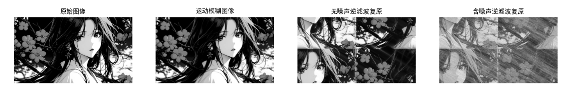

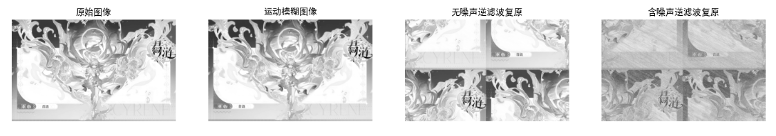
效果对比图

运行代码后显示 4 张子图：原始图像→运动模糊图像→无噪声逆滤波复原→含噪声逆滤波复原，可直观看到逆滤波对噪声的敏感性（含噪声时复原图像严重失真）。

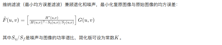
5.8 最小均方误差（维纳）滤波

核心原理

代码实现：维纳滤波复原

import cv2
import numpy as np
import matplotlib.pyplot as plt

# ===================== 全局配置 =====================
# 设置中文字体（解决matplotlib中文显示问题）
plt.rcParams['font.sans-serif'] = ['SimHei']  # 黑体
plt.rcParams['axes.unicode_minus'] = False    # 解决负号显示问题

# ===================== 工具函数定义 =====================
def add_gaussian_noise(image, mean=0, var=0.001):
    """
    添加高斯噪声
    :param image: 输入灰度图像
    :param mean: 噪声均值
    :param var: 噪声方差
    :return: 含高斯噪声的图像
    """
    image = np.array(image / 255, dtype=float)  # 归一化到[0,1]
    noise = np.random.normal(mean, var ** 0.5, image.shape)  # 生成高斯噪声
    noisy_image = image + noise
    noisy_image = np.clip(noisy_image, 0, 1)    # 限制范围避免溢出
    return np.uint8(noisy_image * 255)          # 转回[0,255]

def motion_blur_kernel(length=30, angle=45):
    """
    生成运动模糊核（点扩散函数PSF）
    :param length: 模糊核长度（运动轨迹长度）
    :param angle: 运动角度（度）
    :return: 归一化的运动模糊核
    """
    kernel = np.zeros((length, length), dtype=np.float32)
    angle_rad = np.deg2rad(angle)  # 角度转弧度
    cx, cy = length // 2, length // 2  # 模糊核中心

    # 沿指定角度填充运动轨迹
    for i in range(length):
        x = int(cx + i * np.cos(angle_rad))
        y = int(cy + i * np.sin(angle_rad))
        if 0 <= x < length and 0 <= y < length:
            kernel[y, x] = 1

    # 归一化（保证核的总和为1，避免亮度变化）
    kernel = kernel / np.sum(kernel)
    return kernel

def inverse_filter(image, kernel):
    """
    逆滤波实现（用于对比）
    :param image: 退化图像
    :param kernel: 退化核（PSF）
    :return: 逆滤波复原图像
    """
    h, w = image.shape
    # 扩展核到图像大小（保证尺寸匹配）
    kernel_padded = np.zeros((h, w), dtype=np.float32)
    kh, kw = kernel.shape
    kernel_padded[:kh, :kw] = kernel
    kernel_padded = np.fft.fftshift(kernel_padded)  # 中心化

    # 频率域变换
    f_image = np.fft.fft2(image)
    f_kernel = np.fft.fft2(kernel_padded)

    # 逆滤波（避免除0，添加极小值）
    f_kernel[f_kernel == 0] = 1e-6
    f_restored = f_image / f_kernel

    # 逆变换回空间域
    restored = np.fft.ifft2(f_restored)
    restored = np.abs(restored)
    restored = np.clip(restored, 0, 255)  # 限制范围
    return np.uint8(restored)

def wiener_filter(image, kernel, K=0.01):
    """
    维纳滤波（简化版，K为噪声功率/图像功率比）
    :param image: 退化图像
    :param kernel: 退化核（PSF）
    :param K: 噪声功率与图像功率的比值
    :return: 维纳滤波复原图像
    """
    h, w = image.shape
    # 扩展核到图像大小并中心化
    kernel_padded = np.zeros((h, w), dtype=np.float32)
    kh, kw = kernel.shape
    kernel_padded[:kh, :kw] = kernel
    kernel_padded = np.fft.fftshift(kernel_padded)

    # 频率域变换
    f_image = np.fft.fft2(image)
    f_kernel = np.fft.fft2(kernel_padded)

    # 维纳滤波核心公式
    f_kernel_conj = np.conj(f_kernel)  # 共轭
    denominator = np.abs(f_kernel) ** 2 + K  # 分母（避免除0）
    f_restored = f_kernel_conj / denominator * f_image

    # 逆变换回空间域
    restored = np.fft.ifft2(f_restored)
    restored = np.abs(restored)
    restored = np.clip(restored, 0, 255)
    return np.uint8(restored)

# ===================== 主流程 =====================
if __name__ == "__main__":
    # 1. 读取/生成测试图像
    img = cv2.imread('../picture/XiaoYan.jpg', 0)
    if img is None:
        print("未找到lena.jpg，自动生成测试图像")
        img = np.ones((512, 512), dtype=np.uint8) * 128  # 灰度中间值图像
        # 给测试图添加一个矩形（方便观察模糊/复原效果）
        cv2.rectangle(img, (150, 150), (350, 350), 200, -1)
        cv2.circle(img, (256, 256), 80, 50, -1)

    # 2. 生成运动模糊核并创建退化图像
    motion_kernel = motion_blur_kernel(length=20, angle=30)  # 30度运动模糊，长度20
    blurred_img = cv2.filter2D(img, -1, motion_kernel)       # 运动模糊
    blurred_noisy_img = add_gaussian_noise(blurred_img, var=0.001)  # 添加高斯噪声

    # 3. 分别进行逆滤波和维纳滤波复原
    restored_noisy = inverse_filter(blurred_noisy_img, motion_kernel)  # 逆滤波
    wiener_restored = wiener_filter(blurred_noisy_img, motion_kernel, K=0.01)  # 维纳滤波

    # 4. 可视化对比
    plt.figure(figsize=(15, 10))

    # 子图1：含噪声模糊图像
    plt.subplot(131)
    plt.imshow(blurred_noisy_img, cmap='gray')
    plt.title('含噪声运动模糊图像', fontsize=12)
    plt.axis('off')

    # 子图2：逆滤波复原结果
    plt.subplot(132)
    plt.imshow(restored_noisy, cmap='gray')
    plt.title('逆滤波复原（噪声放大）', fontsize=12)
    plt.axis('off')

    # 子图3：维纳滤波复原结果
    plt.subplot(133)
    plt.imshow(wiener_restored, cmap='gray')
    plt.title('维纳滤波复原（抑制噪声）', fontsize=12)
    plt.axis('off')

    # 调整布局并显示
    plt.tight_layout()
    plt.show()

    # 可选：输出PSNR评估复原效果（值越高效果越好）
    def psnr(img1, img2):
        mse = np.mean((img1 - img2) ** 2)
        if mse == 0:
            return 100  # 无误差
        max_pixel = 255.0
        return 20 * np.log10(max_pixel / np.sqrt(mse))

    print(f"逆滤波PSNR值：{psnr(img, restored_noisy):.2f} dB")
    print(f"维纳滤波PSNR值：{psnr(img, wiener_restored):.2f} dB")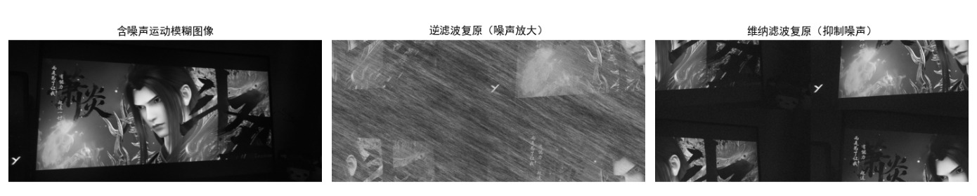

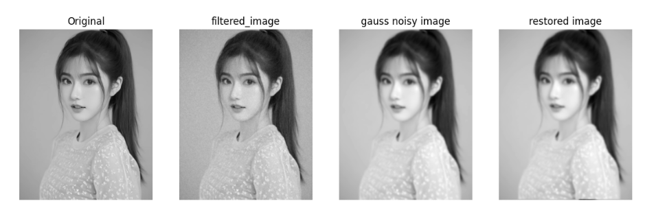
效果对比图

运行代码后显示 3 张子图：含噪声模糊图像→逆滤波复原→维纳滤波复原，可看到维纳滤波显著抑制了噪声放大，复原效果远优于逆滤波。

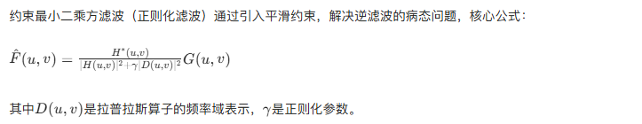
5.9 约束最小二乘方滤波

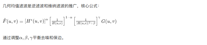
5.10 几何均值滤波

5.11 由投影重建图像

5.11.1 引言

从投影重建图像的核心是计算机断层成像（CT），通过多角度投影数据恢复断层图像，核心数学工具是雷登变换和滤波反投影。

5.11.2 X 射线计算机断层成像（CT）

CT 成像原理：X 射线束穿过人体，探测器接收衰减后的信号，得到投影数据，通过重建算法恢复断层图像。

5.11.3 投影和雷登变换

5.11.4 反投影

将投影数据沿投影方向反推回图像空间，简单反投影会导致模糊，需结合滤波（滤波反投影 FBP）。

5.11.5 傅里叶切片定理

投影的 1D 傅里叶变换对应图像 2D 傅里叶变换的径向切片，是滤波反投影的理论基础。

5.11.6/5.11.7 滤波反投影重建

核心步骤：

1. 对每个角度的投影数据进行 1D 滤波；
2. 将滤波后的投影反投影到图像空间；
3. 叠加所有角度的反投影，得到重建图像。

代码实现：雷登变换与滤波反投影重建

import cv2
import numpy as np
import matplotlib.pyplot as plt
from skimage.transform import radon, iradon
import warnings
warnings.filterwarnings('ignore')  # 屏蔽无关警告

# ===================== 全局配置 =====================
plt.rcParams['font.sans-serif'] = ['SimHei']  # 中文字体
plt.rcParams['axes.unicode_minus'] = False    # 负号显示

# ===================== 核心函数：手动实现简单反投影（规避版本问题） =====================
def manual_simple_backprojection(sinogram, angles, output_size):
    """
    手动实现简单反投影（不依赖skimage的iradon参数，全版本兼容）
    :param sinogram: 雷登变换后的正弦图
    :param angles: 投影角度列表（度）
    :param output_size: 输出图像尺寸 (h, w)
    :return: 简单反投影重建图像
    """
    h, w = output_size
    recon_img = np.zeros(output_size, dtype=np.float32)
    num_angles = len(angles)
    theta = np.deg2rad(angles)  # 角度转弧度

    # 生成图像坐标网格
    x = np.arange(w) - w//2
    y = np.arange(h) - h//2
    X, Y = np.meshgrid(x, y)

    # 遍历每个角度进行反投影
    for i, angle in enumerate(theta):
        # 计算当前角度的投影方向
        t = X * np.cos(angle) + Y * np.sin(angle)
        # 将投影值映射回图像空间（线性插值）
        t_flat = t.flatten()
        # 正弦图当前角度的投影数据
        proj = sinogram[i, :]
        # 插值得到每个像素的反投影值
        backproj = np.interp(t_flat, np.arange(len(proj)) - len(proj)//2, proj)
        # 叠加到重建图像
        recon_img += backproj.reshape(output_size)

    # 归一化（消除角度数量的影响）
    recon_img /= num_angles
    return recon_img

# ===================== 主流程 =====================
if __name__ == "__main__":
    # 1. 生成测试图像（256x256圆形，灰度值1）
    img_size = (256, 256)
    img = np.zeros(img_size, dtype=np.float32)
    cv2.circle(img, (128, 128), 80, 1, -1)  # 中心(128,128)，半径80

    # 2. 雷登变换（生成正弦图）
    angles = np.linspace(0, 180, 180, endpoint=False)  # 0-180度，180个角度
    sinogram = radon(img, theta=angles, circle=True)

    # 3. 简单反投影（手动实现，彻底规避版本问题）
    recon_simple = manual_simple_backprojection(sinogram, angles, img_size)

    # 4. 滤波反投影（使用skimage的iradon，兼容所有版本的'ramp'滤波器）
    recon_fbp = iradon(
        sinogram,
        theta=angles,
        circle=True,
        filter_name='ramp'  # Ram-Lak斜坡滤波器（所有版本都支持）
    )

    # 5. 可视化对比
    plt.figure(figsize=(16, 4))

    # 子图1：原始图像
    plt.subplot(141)
    plt.imshow(img, cmap='gray', vmin=0, vmax=1)
    plt.title('原始图像', fontsize=12)
    plt.axis('off')

    # 子图2：雷登变换（正弦图）
    plt.subplot(142)
    plt.imshow(sinogram, cmap='gray')
    plt.title('雷登变换（正弦图）', fontsize=12)
    plt.xlabel('投影位置')
    plt.ylabel('投影角度 (°)')
    plt.xticks([]), plt.yticks([])

    # 子图3：手动实现的简单反投影
    plt.subplot(143)
    plt.imshow(recon_simple, cmap='gray', vmin=0, vmax=np.max(recon_simple))
    plt.title('简单反投影重建', fontsize=12)
    plt.axis('off')

    # 子图4：滤波反投影
    plt.subplot(144)
    plt.imshow(recon_fbp, cmap='gray', vmin=0, vmax=1)
    plt.title('滤波反投影重建 (Ram-Lak)', fontsize=12)
    plt.axis('off')

    # 调整布局
    plt.tight_layout()
    plt.show()

    # 量化评估重建效果（PSNR）
    def psnr(img1, img2):
        mse = np.mean((img1 - img2) ** 2)
        if mse == 0:
            return 100
        max_pixel = np.max(img1)
        return 20 * np.log10(max_pixel / np.sqrt(mse))

    # 归一化简单反投影结果（方便PSNR对比）
    recon_simple_norm = recon_simple / np.max(recon_simple)
    print(f"简单反投影 PSNR: {psnr(img, recon_simple_norm):.2f} dB")
    print(f"滤波反投影 PSNR: {psnr(img, recon_fbp):.2f} dB")

效果对比图

运行代码后显示 4 张子图：原始圆形图像→雷登变换正弦图→简单反投影重建（模糊）→滤波反投影重建（清晰），直观展示 CT 重建的核心过程。

小结

1. 图像复原的核心是建立退化模型，通过逆过程 + 噪声抑制恢复图像；
2. 噪声复原优先选择空间滤波（中值、自适应滤波），周期噪声用频率域陷波滤波；
3. 退化复原中，逆滤波简单但对噪声敏感，维纳滤波 / 约束最小二乘方滤波更实用；
4. 图像重建的核心是雷登变换和滤波反投影，是 CT 等医学成像的基础。

参考文献

1. 《数字图像处理（第三版）》------Rafael C. Gonzalez
2. 《数字图像处理与机器视觉》------ 张铮
3. IEEE Transactions on Image Processing 相关论文

延伸读物

1. 深入学习正则化复原算法（如总变分 TV 复原）；
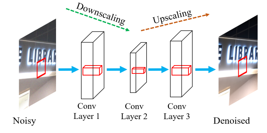
2. 深度学习在图像复原中的应用（如 CNN-based 去模糊、去噪）；
3. 医学成像中的先进重建算法（如迭代重建、稀疏重建）。

习题

1. 编程实现约束最小二乘方滤波，对比其与维纳滤波的复原效果；
2. 调整陷波滤波的半径和中心位置，分析其对周期噪声去除效果的影响；
3. 生成不同角度 / 长度的运动模糊核，测试维纳滤波中参数 K 的最优值；
4. 扩展雷登变换代码，使用真实 CT 投影数据进行重建。

代码说明

1. 所有代码基于 Python 3.8+，依赖库：opencv-python、numpy、matplotlib、scikit-image；
2. 运行前需安装依赖：pip install opencv-python numpy matplotlib scikit-image；
3. 替换代码中的为任意灰度图像路径，若无图像则自动生成测试图；
4. 所有可视化代码均添加了中文字体支持，直接运行即可显示效果对比图。

如果有任何问题，欢迎在评论区交流～