遗传算法学习二之求TSP问题

目录

前言

一、TSP问题？

问题描述：

[1. 精确算法 (获得全局最优解)](#1. 精确算法 (获得全局最优解))

[2. 启发式与元启发式算法 (获得近似最优解)](#2. 启发式与元启发式算法 (获得近似最优解))

二、算法实现

2.1、个体编码

2.2、初始种群

2.3、计算适应度

2.4、选择操作

2.5、交叉操作

2.6、变异操作

2.7、生成新种群

三、整体代码

四、结果查看

---

前言

本章会用最基础的函数基于遗传算法求解TSP问题，遗传算法里的编码、群体设定、适应度函数、选择、交叉和变异都会涉及到。主体代码是AI生成再加上自行修改的

---

一、 TSP问题 ？

TSP 问题（旅行商问题，Traveling Salesman Problem） 是组合优化中的一个经典 NP 难问题，广泛应用于运筹学、计算机科学和物流规划等领域。

问题描述：

给定 n 个城市 和每对城市之间的距离（或代价） ，要求找出一条最短的闭合路径（回路），使得旅行商：

• 从某个城市出发；
• 恰好访问每个城市一次；
• 最后回到起点城市。

下面是比较常用的求解方法。

1. 精确算法 (获得全局最优解)

2. 启发式与元启发式算法 (获得近似最优解)

我们要用的遗传算法在大小规模质量和速度都特别好的方法。下面来看看如何使用

二、算法实现

建议大家先阅读一下遗传算法的思想，理解这个算法本身的含义。下面我按照遗传算法的流程对代码进行分解，方便大家阅读。

2.1、个体编码

也就是对种群中每一个个体信息用数据表示出来，我们这里用实数编码。比如说有5个城市编码成1、2、3、4、5。那么其中一个个体可设为a = [5、3、1、4、2]。这个数组代表的就是旅行商对城市的访问顺序。这就完成了编码。

2.2、初始种群

一个种群是由很多个同类个体组成的。

    nCities = 10; % 城市数量
    cities = 10*rand(nCities, 2); % 随机生成城市坐标
    % 2. 遗传算法参数设置
    popSize = 100; % 种群大小
    % 3. 初始化种群
    population = cell(popSize, 1);
    for i = 1:popSize
        % 每个个体是城市的随机排列
        population{i} = randperm(nCities);
    end

先定义城市数量nCities，随机生成城市坐标cities。这样问题信息就完善了。接着定义种群大小popSize，代表着这个种群中个体的数量。

randperm(nCities)：会返回从 1 到 nCities没有重复元素的整数随机排列。也就是生成了一个个体。for循环生成100个个体组成种群population。

2.3、计算适应度

遗传算法遵循自然界优胜劣退的原则，适应度用来表示个体的优劣。适应度越高别选择繁衍的几率就越大。

   fitness = zeros(popSize, 1);
    for i = 1:popSize
        fitness(i) = calculate_fitness(population{i}, cities);
    end
%*********************************************************
  %功能：适应度计算函数
  %调用格式：fit = calculate_fitness(route, cities)
  %输入参数：route:个体排列顺序，cities：个体坐标
  %输出参数：fit:总路程的倒数（距离越短，适应度越高）
%*********************************************************
function fit = calculate_fitness(route, cities)
    % 计算路径总长度
    totalDist = 0;
    n = length(route);
    for i = 1:n-1
        totalDist = totalDist + norm(cities(route(i),:) - cities(route(i+1),:));
    end
    % 返回终点到起点的距离
    totalDist = totalDist + norm(cities(route(n),:) - cities(route(1),:));
    
    % 适应度为总距离的倒数（距离越短，适应度越高）
    fit = 1/totalDist;
end

用fitness来记录每个个体的适应度值。norm(a,b)：用来计算向量ab的模。

因为前面有了每个城市的坐标点，只需要把每两个坐标点相减再计算模长就得到了两个城市间的距离，依次进行，从而得到一个个体的路程。再将路程取倒数，作为适应度值。

2.4、选择操作

newPopulation = selection(population, fitness, popSize);
%*********************************************************
  %功能：选择操作 - 轮盘赌选择
  %调用格式：newPop = selection(population, fitness, popSize)
  %输入参数：population:初始种群，fitness：适应度函数，popSize：种群大小
  %输出参数：newPop:选择后存活的种群（类别代表存活，个数代表优势）
%*********************************************************
function newPop = selection(population, fitness, popSize)
    % 计算选择概率
    totalFitness = sum(fitness);
    prob = fitness / totalFitness;
    
    % 计算累积概率
    cumProb = cumsum(prob);
    
    % 轮盘赌选择
    newPop = cell(popSize, 1);
    for i = 1:popSize
        r = rand();
        % 找到第一个累积概率大于r的索引
        idx = find(cumProb >= r, 1, 'first');
        newPop{i} = population{idx};
    end
end

计算出每个个体适应度在种群中的概率prob。

cumsum(prob)：返回prob的每一位累积和，也就是[prob(1)、prob(1)+prob(2)、prob(1)+prob(2)+prob(3）.....]。

随机生成一个0-1的值，如果某个下标的累计值大于这个随机值就选中该下标对应的个体遗传下去，共选择100个。在概率上这100中会汇聚更多适应度高的个体。

2.5、交叉操作

    pc = 0.9; % 交叉概率
    for i = 1:2:popSize-1
            if rand() < pc
                [newPopulation{i}, newPopulation{i+1}] = ox_crossover(newPopulation{i}, newPopulation{i+1});
            end
        end
%*********************************************************
  %功能：交叉操作 - 顺序交叉 (Order Crossover, OX)
  %调用格式：[child1, child2] = ox_crossover(parent1, parent2)
  %输入参数：parent1:父代1，parent2：父代2
  %输出参数：[child1, child2]：子代1，子代2，向量形式返回
%*********************************************************
function [child1, child2] = ox_crossover(parent1, parent2)
    n = length(parent1);
    
    % 随机选择两个交叉点
    cp1 = randi([1, n-1]);%随机返回[1, n-1]区间的标量整数
    cp2 = randi([cp1+1, n]);
    
    % 初始化子代
    child1 = zeros(1, n);
    child2 = zeros(1, n);
    
    % 保留中间段
    child1(cp1:cp2) = parent1(cp1:cp2);
    child2(cp1:cp2) = parent2(cp1:cp2);
    
    % 填充child1
    idx = cp2 + 1;
    if idx > n
        idx = 1;
    end
    
    pIdx = cp2 + 1;
    if pIdx > n
        pIdx = 1;
    end
    
    % 从parent2中按顺序填充child1
    while any(child1 == 0)%当child1所有元素非零时返回逻辑0
        val = parent2(pIdx);
        if ~ismember(val, child1)%如果child1中含有val，返回0
            child1(idx) = val;
            idx = idx + 1;
            if idx > n
                idx = 1;
            end
        end
        pIdx = pIdx + 1;
        if pIdx > n
            pIdx = 1;
        end
    end
    
    % 填充child2
    idx = cp2 + 1;
    if idx > n
        idx = 1;
    end
    
    pIdx = cp2 + 1;
    if pIdx > n
        pIdx = 1;
    end
    
    % 从parent1中按顺序填充child2
    while any(child2 == 0)
        val = parent1(pIdx);
        if ~ismember(val, child2)
            child2(idx) = val;
            idx = idx + 1;
            if idx > n
                idx = 1;
            end
        end
        pIdx = pIdx + 1;
        if pIdx > n
            pIdx = 1;
        end
    end
end

当两个生物体配对时，他们的染色体相互混合，产生一对由双方基因组成的新的染色体，这一过程称为交叉。我们这里采用的是顺序交叉

2.6、变异操作

       pm = 0.1; % 变异概率
       for i = 1:popSize
            if rand() < pm
                newPopulation{i} = inversion_mutation(newPopulation{i});
            end
        end
%*********************************************************
  %功能：变异操作 - 逆转变异
  %调用格式：mutatedRoute = inversion_mutation(route)
  %输入参数：route:待变异个体
  %输出参数：mutatedRoute：变异后的个体
%*********************************************************
function mutatedRoute = inversion_mutation(route)
    n = length(route);
    
    % 随机选择两个点
    idx1 = randi([1, n-1]);
    idx2 = randi([idx1+1, n]);
    
    % 逆转变异：将idx1到idx2之间的城市顺序反转
    mutatedRoute = route;
    mutatedRoute(idx1:idx2) = fliplr(route(idx1:idx2));
end

2.7、生成新种群

        % 计算新种群的适应度
        newFitness = zeros(popSize, 1);
        for i = 1:popSize
            newFitness(i) = calculate_fitness(newPopulation{i}, cities);
        end
        
        % 6.5 精英策略 - 保留最优个体
        [~, bestIdx] = max(fitness);  % 适应度最高的个体索引
        [~, worstIdxNew] = min(newFitness);  % 新种群中适应度最低的个体索引
        
        % 用旧种群的最优个体替换新种群的最差个体
        newPopulation{worstIdxNew} = population{bestIdx};
        newFitness(worstIdxNew) = fitness(bestIdx);
        
        % 6.6 更新种群
        population = newPopulation;
        fitness = newFitness;

经过前面的步骤就完成了一次迭代产生了新的种群，再继续往复迭代下去。这样就能找到最优解了。

三、整体代码

    clear; close;
    rng default  %固定随机种子（保证结果可复现）
    nCities = 10; % 城市数量
    cities = 10*rand(nCities, 2); % 随机生成城市坐标
    
    % 2. 遗传算法参数设置
    popSize = 100; % 种群大小
    maxGen = 500; % 最大迭代代数
    pc = 0.9; % 交叉概率
    pm = 0.1; % 变异概率
    
    % 3. 初始化种群
    population = cell(popSize, 1);
    for i = 1:popSize
        % 每个个体是城市的随机排列
        population{i} = randperm(nCities);
    end
    
    % 4. 计算初始适应度
    fitness = zeros(popSize, 1);
    for i = 1:popSize
        fitness(i) = calculate_fitness(population{i}, cities);
    end
    
    % 5. 记录每代的最佳个体
    bestFitness = zeros(maxGen, 1);%最佳适应度
    bestSolution = zeros(1, nCities);%最佳个体
    bestDistance = inf;%最佳路程距离
    
    % 6. 遗传算法主循环
    for gen = 1:maxGen
        % 6.1 选择操作 - 轮盘赌选择
        newPopulation = selection(population, fitness, popSize);
        
        % 6.2 交叉操作 - 顺序交叉 (OX)
        for i = 1:2:popSize-1
            if rand() < pc
                [newPopulation{i}, newPopulation{i+1}] = ox_crossover(newPopulation{i}, newPopulation{i+1});
            end
        end
        
        % 6.3 变异操作 - 逆转变异
        for i = 1:popSize
            if rand() < pm
                newPopulation{i} = inversion_mutation(newPopulation{i});
            end
        end
        
        % 6.4 计算新种群的适应度
        newFitness = zeros(popSize, 1);
        for i = 1:popSize
            newFitness(i) = calculate_fitness(newPopulation{i}, cities);
        end
        
        % 6.5 精英策略 - 保留最优个体
        [~, bestIdx] = max(fitness);  % 适应度最高的个体索引
        [~, worstIdxNew] = min(newFitness);  % 新种群中适应度最低的个体索引
        
        % 用旧种群的最优个体替换新种群的最差个体
        newPopulation{worstIdxNew} = population{bestIdx};
        newFitness(worstIdxNew) = fitness(bestIdx);
        
        % 6.6 更新种群
        population = newPopulation;
        fitness = newFitness;
        
        % 6.7 记录最佳解
        [maxFit, idx] = max(fitness);
        bestFitness(gen) = maxFit;
        bestDistance = 1/maxFit;
        bestSolution = population{idx};
        
        % 6.8 显示进度
        if mod(gen, 50) == 0
            fprintf('Generation %d: Best distance = %.4f\n', gen, bestDistance);
        end
    end
    
    % 7. 结果可视化
    plot_tsp_solution(cities, bestSolution, bestDistance);
    
    % 8. 绘制适应度变化曲线
    figure(2);
    set(gcf,"Theme","dark");
    plot(1:maxGen, 1./bestFitness, 'LineWidth', 1.5);
    xlabel('Generation');
    ylabel('Best Distance');
    title('Genetic Algorithm Convergence');
    grid on;
    
    fprintf('Optimization complete. Best distance: %.4f\n', bestDistance);

%*********************************************************
  %功能：适应度计算函数
  %调用格式：fit = calculate_fitness(route, cities)
  %输入参数：route:个体排列顺序，cities：个体坐标
  %输出参数：fit:总路程的倒数（距离越短，适应度越高）
%*********************************************************
function fit = calculate_fitness(route, cities)
    % 计算路径总长度
    totalDist = 0;
    n = length(route);
    for i = 1:n-1
        totalDist = totalDist + norm(cities(route(i),:) - cities(route(i+1),:));
    end
    % 返回终点到起点的距离
    totalDist = totalDist + norm(cities(route(n),:) - cities(route(1),:));
    
    % 适应度为总距离的倒数（距离越短，适应度越高）
    fit = 1/totalDist;
end

%*********************************************************
  %功能：选择操作 - 轮盘赌选择
  %调用格式：newPop = selection(population, fitness, popSize)
  %输入参数：population:初始种群，fitness：适应度函数，popSize：种群大小
  %输出参数：newPop:选择后存活的种群（类别代表存活，个数代表优势）
%*********************************************************
function newPop = selection(population, fitness, popSize)
    % 计算选择概率
    totalFitness = sum(fitness);
    prob = fitness / totalFitness;
    
    % 计算累积概率
    cumProb = cumsum(prob);
    
    % 轮盘赌选择
    newPop = cell(popSize, 1);
    for i = 1:popSize
        r = rand();
        % 找到第一个累积概率大于r的索引
        idx = find(cumProb >= r, 1, 'first');
        newPop{i} = population{idx};
    end
end

%*********************************************************
  %功能：交叉操作 - 顺序交叉 (Order Crossover, OX)
  %调用格式：[child1, child2] = ox_crossover(parent1, parent2)
  %输入参数：parent1:父代1，parent2：父代2
  %输出参数：[child1, child2]：子代1，子代2，向量形式返回
%*********************************************************
function [child1, child2] = ox_crossover(parent1, parent2)
    n = length(parent1);
    
    % 随机选择两个交叉点
    cp1 = randi([1, n-1]);%随机返回[1, n-1]区间的标量整数
    cp2 = randi([cp1+1, n]);
    
    % 初始化子代
    child1 = zeros(1, n);
    child2 = zeros(1, n);
    
    % 保留中间段
    child1(cp1:cp2) = parent1(cp1:cp2);
    child2(cp1:cp2) = parent2(cp1:cp2);
    
    % 填充child1
    idx = cp2 + 1;
    if idx > n
        idx = 1;
    end
    
    pIdx = cp2 + 1;
    if pIdx > n
        pIdx = 1;
    end
    
    % 从parent2中按顺序填充child1
    while any(child1 == 0)%当child1所有元素非零时返回逻辑0
        val = parent2(pIdx);
        if ~ismember(val, child1)%如果child1中含有val，返回0
            child1(idx) = val;
            idx = idx + 1;
            if idx > n
                idx = 1;
            end
        end
        pIdx = pIdx + 1;
        if pIdx > n
            pIdx = 1;
        end
    end
    
    % 填充child2
    idx = cp2 + 1;
    if idx > n
        idx = 1;
    end
    
    pIdx = cp2 + 1;
    if pIdx > n
        pIdx = 1;
    end
    
    % 从parent1中按顺序填充child2
    while any(child2 == 0)
        val = parent1(pIdx);
        if ~ismember(val, child2)
            child2(idx) = val;
            idx = idx + 1;
            if idx > n
                idx = 1;
            end
        end
        pIdx = pIdx + 1;
        if pIdx > n
            pIdx = 1;
        end
    end
end

%*********************************************************
  %功能：变异操作 - 逆转变异
  %调用格式：mutatedRoute = inversion_mutation(route)
  %输入参数：route:待变异个体
  %输出参数：mutatedRoute：变异后的个体
%*********************************************************
function mutatedRoute = inversion_mutation(route)
    n = length(route);
    
    % 随机选择两个点
    idx1 = randi([1, n-1]);
    idx2 = randi([idx1+1, n]);
    
    % 逆转变异：将idx1到idx2之间的城市顺序反转
    mutatedRoute = route;
    mutatedRoute(idx1:idx2) = fliplr(route(idx1:idx2));
end

%*********************************************************
  %功能：绘制TSP解决方案
  %调用格式：plot_tsp_solution(cities, bestRoute, bestDistance)
  %输入参数：cities:城市坐标，bestRoute：最佳个体，bestDistance：最佳路程距离
  %输出参数：mutatedRoute：变异后的个体
%*********************************************************
function plot_tsp_solution(cities, bestRoute, bestDistance)
    figure(1);
    set(gcf,"Theme","dark");
    hold on;
    grid on;
    
    % 绘制城市点
    scatter(cities(:,1), cities(:,2), 50,"filled");
    
    % 绘制路径
    n = length(bestRoute);
    for i = 1:n-1
        plot([cities(bestRoute(i),1), cities(bestRoute(i+1),1)], ...
             [cities(bestRoute(i),2), cities(bestRoute(i+1),2)], 'r-', 'LineWidth', 1.5);
    end
    % 连接最后一个城市和第一个城市
    plot([cities(bestRoute(n),1), cities(bestRoute(1),1)], ...
         [cities(bestRoute(n),2), cities(bestRoute(1),2)], 'r-', 'LineWidth', 1.5);
    
    % 标记起点和终点
    scatter(cities(bestRoute(1),1), cities(bestRoute(1),2), 100,"filled", "green");
    scatter(cities(bestRoute(n),1), cities(bestRoute(n),2), 100, "filled","cyan");
    
    % 添加标题和标签
    title(sprintf('TSP Solution using Genetic Algorithm (Distance = %.4f)', bestDistance));
    xlabel('X Coordinate');
    ylabel('Y Coordinate');
    
    % 为每个城市添加编号
    for i = 1:size(cities, 1)
        text(cities(i,1)-0.1, cities(i,2)-0.1, num2str(i), 'FontSize', 12);
    end
    text(cities(bestRoute(1),1)+0.1, cities(bestRoute(1),2)+0.1, "起始点", 'FontSize', 12);
    text(cities(bestRoute(n),1)+0.1, cities(bestRoute(n),2)+0.1, "终止点", 'FontSize', 12);
    
    hold off;
end

四、结果查看

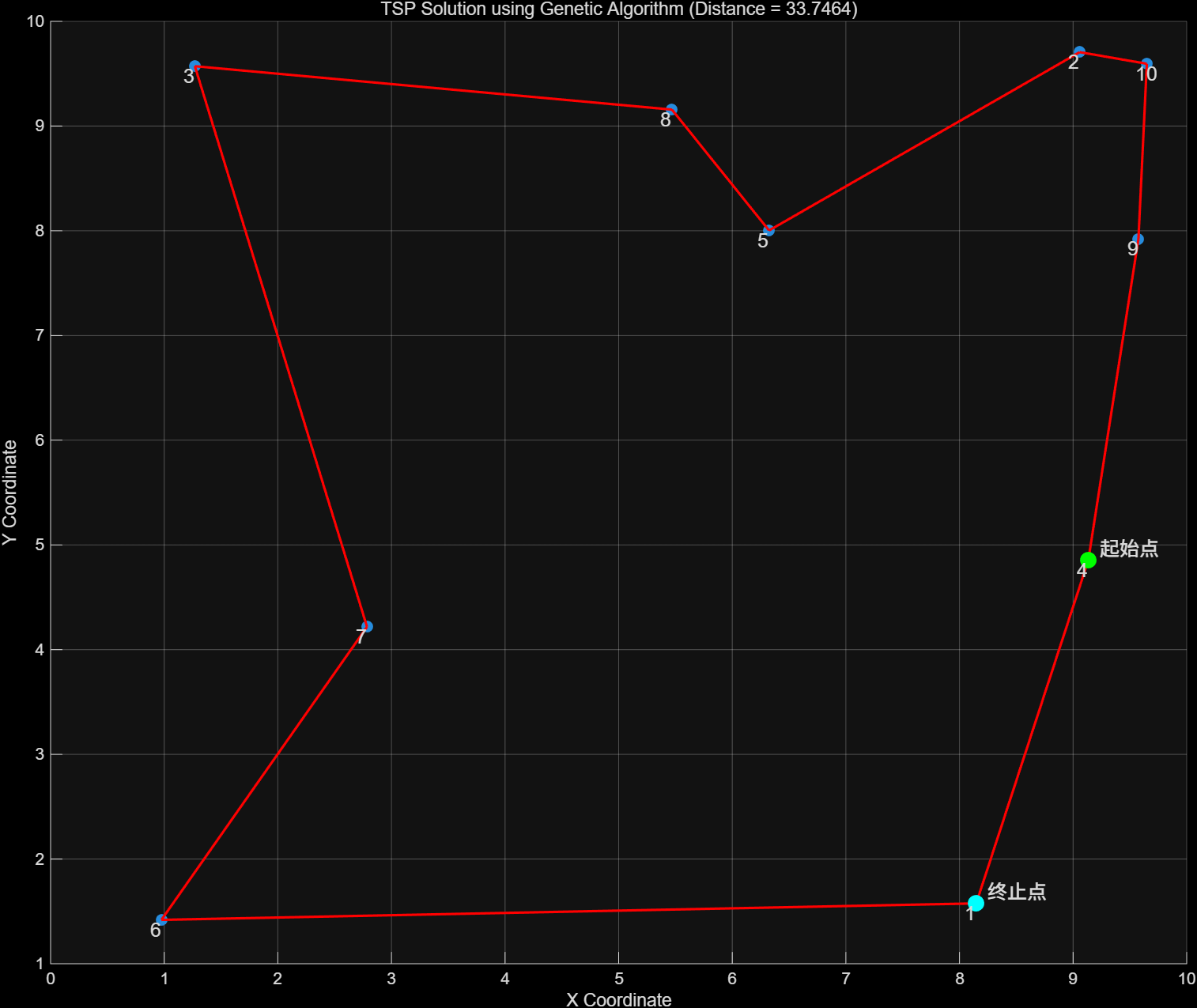
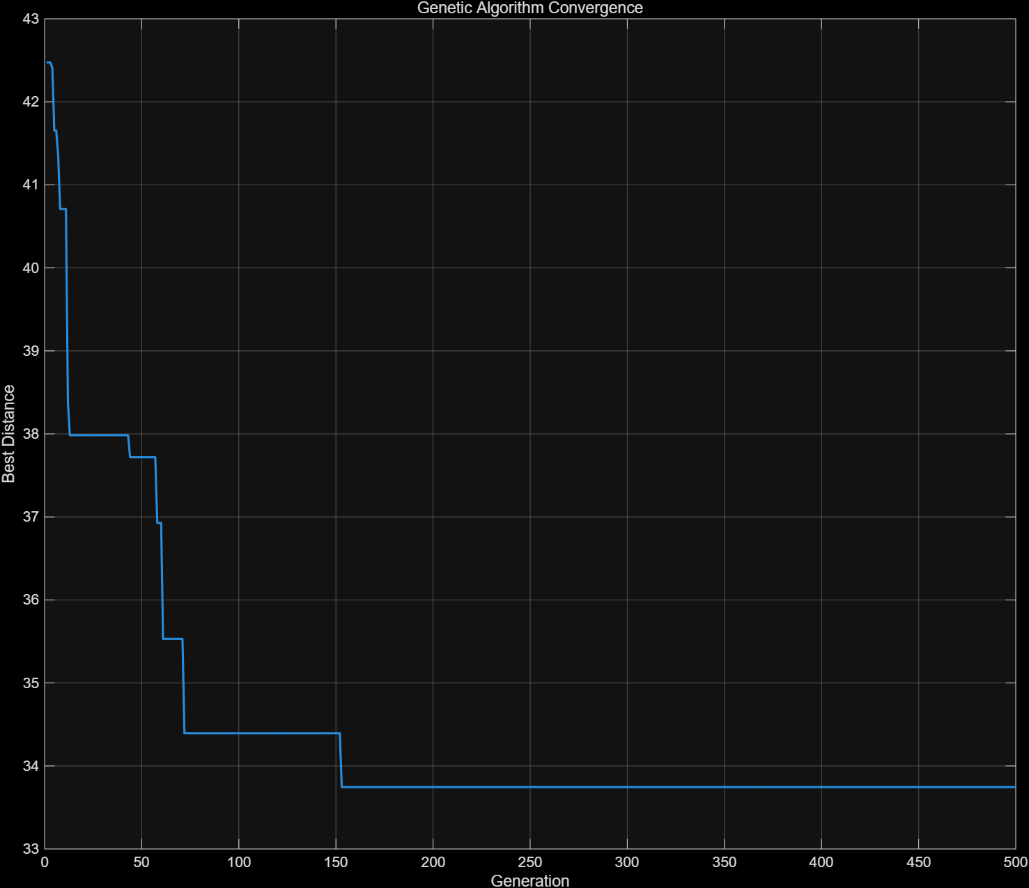
第一张图片是城市路径，总距离为33.7464。第二张图是总路程的迭代图，可以看到大概在160次迭代后找到了最优解