文章目录
-
- 摘要
- Abstract
-
- [1.1 传统优化算法](#1.1 传统优化算法)
- 1.2高纬度多目标优化算法
- 总结
摘要
本周学习了传统优化算法在高纬度失效的场景,并且实现了基于分解的MOEA/D-DRA算法来适应高纬度优化。
Abstract
This week, we studied the scenarios where traditional optimization algorithms fail in high-dimensional spaces and implemented the decomposition-based MOEA/D-DRA algorithm to adapt to high-dimensional optimization.
1.1 传统优化算法
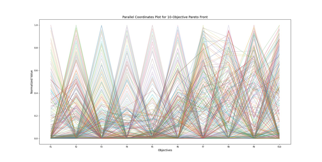
NSGA-II在高纬度时, 以上是NGSA-II在目标维度是10,种群大小为300,迭代250次之后得到的最终结果,发现NGSA-II的帕累托更杂乱,解没有收敛到清晰的帕累托前沿,而是均匀地、随机地散布在整个目标空间的中间区域。几乎所有线条都穿过了每个目标从0到1的几乎所有值。这意味着很多解在各个目标上都表现平庸,且互相之间不构成明显的支配关系。
1.2高纬度多目标优化算法
MOEA/D-DRA 的核心思想是将 10 目标优化问题分解为多个单目标子问题,通过动态分配搜索资源提升整体优化效果,具体机制如下:
问题分解机制
MOEA/D-DRA 是在 MOEA/D 框架基础上发展而来的改进版本。MOEA/D 通过将多目标问题分解为多个标量子问题,并利用一组均匀分布的权重向量来引导搜索方向。每个子问题对应一个权重向量,并通过聚合函数(如 Tchebycheff 函数)将多目标问题转化为单目标问题:

其中w是权重向量,z^*为理想点。
与标准 MOEA/D 不同,MOEA/D-DRA 引入了动态资源分配机制,即根据子问题的"效用"动态选择一部分子问题进行演化,而不是对所有子问题一视同仁。这种机制的核心在于:
效用函数定义:每个子问题的效用π^i反映了其在最近若干代中的改进程度。具体定义为:
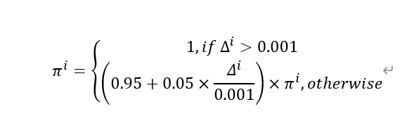
其中Δ^i 是子问题i的适应度改进率,计算如下:
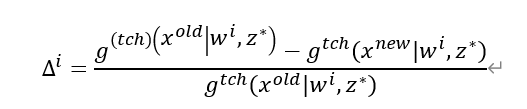
该值越大,说明该子问题在最近的优化中获得了更大的改进,因此更值得投入计算资源。
资源分配策略:在每一代中,算法根据效用值对所有子问题进行排序,优先选择效用高的子问题进行繁殖和更新。这种策略可以有效集中计算资源于"有潜力"的搜索区域,从而提升整体收敛速度和解集质量。
动态资源分配(DRA)
效用评估:根据子问题的历史改进情况计算效用值,反映子问题的优化潜力;
资源倾斜:将搜索资源优先分配给效用值高的子问题,提高搜索效率;
休眠激活:定期激活效用值过低的 "休眠" 子问题,避免算法早熟收敛。
邻域协作机制
为每个子问题构建邻域结构(基于权重向量的欧氏距离);
子问题的演化仅在其邻域内选择父代,保持解的局部一致性;
通过邻域更新实现子问题间的信息共享,促进帕累托前沿的整体推进。
python
import random

import numpy as np
from matplotlib import pyplot as plt
import pandas as pd
np.random.seed(42)
random.seed(42)


def dtlz1(x, m):
    x = np.asarray(x)
    n = len(x)
    k = n - m + 1
    assert k >= 1, "n must be >= m"
    g = 100 * (k + np.sum((x[-k:] - 0.5) ** 2 - np.cos(20 * np.pi * (x[-k:] - 0.5))))
    f = []
    for i in range(m):
        fi = 0.5 * (1 + g)
        for j in range(m - i - 1):
            fi *= x[j]
        if i > 0:
            fi *= (1 - x[m - i - 1])
        f.append(fi)
    return np.array(f)


def fast_non_dominated_sort(objectives):
    objectives = np.array(objectives)
    n = objectives.shape[0]
    domination_count = np.zeros(n, dtype=int)
    # 被支配的集合
    dominated_set = [[] for _ in range(n)]
    # 前沿列表
    fronts = []

    for i in range(n):
        for j in range(n):
            if i == j:
                continue
            # 检查i是否支配j
            if np.all(objectives[i] <= objectives[j]) and np.any(objectives[i] < objectives[j]):
                dominated_set[i].append(j)
            # 检查j是否支配i
            elif np.all(objectives[j] <= objectives[i]) and np.any(objectives[j] < objectives[i]):
                domination_count[i] += 1
    # 找到第一前沿(非支配解)
    current_front = [i for i in range(n) if domination_count[i] == 0]
    fronts.append(current_front)

    # 寻找后续前沿
    while current_front:
        next_front = []
        for i in current_front:
            for j in dominated_set[i]:
                domination_count[j] -= 1
                if domination_count[j] == 0:
                    next_front.append(j)
        if next_front:
            fronts.append(next_front)
        current_front = next_front

    return fronts


def crowed_distance_assignment(objectives):
    pop_size, num_objectives = objectives.shape
    distances = np.zeros(pop_size)

    for m in range(num_objectives):
        indices = np.argsort(objectives[:, m])
        distances[indices[0]] = np.inf  # 边界个体
        distances[indices[-1]] = np.inf  # 边界个体
        norm = objectives[indices[-1], m] - objectives[indices[0], m]

        if norm == 0: continue  # 如果所有目标值相同,则跳过

        for i in range(1, pop_size - 1):
            distances[indices[i]] += (objectives[indices[i + 1], m] - objectives[indices[i - 1], m]) / norm

    return distances


def sbx_crossover(parent1, parent2, eta, bounds, crossover_rate=1.0):
    if random.random() > crossover_rate:
        return np.array(parent1), np.array(parent2)

    parent1 = np.array(parent1)
    parent2 = np.array(parent2)
    vars = len(parent1)
    child1 = np.copy(parent1)
    child2 = np.copy(parent2)

    for i in range(vars):
        x1 = parent1[i]
        x2 = parent2[i]
        low, high = bounds[i]

        if abs(x1 - x2) < 1e-14:
            child1[i] = x1
            child2[i] = x2
            continue
        if x1 > x2:
            x1, x2 = x2, x1
            swapped = True
        else:
            swapped = False
        u = random.random()
        if u <= 0.5:
            beta = (2.0 * u) ** (1.0 / (eta + 1.0))
        else:
            beta = (1.0 / (2.0 * (1.0 - u))) ** (1.0 / (eta + 1.0))
        c1 = 0.5 * ((1 + beta) * x1 + (1 - beta) * x2)
        c2 = 0.5 * ((1 - beta) * x1 + (1 + beta) * x2)

        c1 = np.clip(c1, low, high)
        c2 = np.clip(c2, low, high)

        if swapped:
            child1[i] = c2
            child2[i] = c1
        else:
            child1[i] = c1
            child2[i] = c2

    return child1, child2


def polynomial_mutation(entry, bounds, mutation_rate=1.0, eta=20):
    individual = np.array(entry, dtype=float)
    mutated = np.copy(individual)
    n = len(individual)

    for i in range(n):
        if random.random() >= mutation_rate:
            continue

        low, high = bounds[i]
        y = mutated[i]

        u = random.random()
        if u <= 0.5:
            delta = (2 * u) ** (1.0 / (eta + 1)) - 1.0
        else:
            delta = 1.0 - (2 * (1 - u)) ** (1.0 / (eta + 1))

        y_new = y + delta * (high - low)
        y_new = np.clip(y_new, low, high)
        mutated[i] = y_new

    return mutated


def binary_tournament_selection(population, rank, crowding_distances):
    pop_size = len(population)
    idx1, idx2 = np.random.choice(pop_size, 2, replace=False)

    # 优先选择rank小的
    if rank[idx1] < rank[idx2]:
        return population[idx1]
    elif rank[idx1] > rank[idx2]:
        return population[idx2]
    else:
        # rank相同,选择拥挤距离大的
        if crowding_distances[idx1] > crowding_distances[idx2]:
            return population[idx1]
        else:
            return population[idx2]


def generate_weight(N, m):
    return np.random.dirichlet(np.ones(m), size=N)


def tchebycheff(y, weight, z):
    return np.max(weight * np.abs(y - z))


def differential_evolution(parent1, parent2, parent3, F=0.5):
    parent1 = np.array(parent1)
    parent2 = np.array(parent2)
    parent3 = np.array(parent3)
    # 基本差分变异
    mutant = parent1 + F * (parent2 - parent3)
    return mutant


def compute_utility(old_objs, new_objs, weights, z, delta=1e-8):
    old_val = tchebycheff(old_objs, weights, z)
    new_val = tchebycheff(new_objs, weights, z)

    if abs(old_val) < delta:
        return 0.0

    improvement = (old_val - new_val) / old_val
    return max(0.0, improvement)  # 只考虑改进


# 动态资源分配选择
def dra_selection(pi, k):
    n = len(pi)
    k = min(k, n)
    norm = pi + 1e-10
    pi_min, pi_max = norm.min(), norm.max()

    if pi_max - pi_min > 1e-10:
        pi_norm = (norm - pi_min) / (pi_max - pi_min)
    else:
        pi_norm = np.ones(n)

    p = pi_norm / pi_norm.sum()
    if np.any(np.isnan(p)) or np.any(p < 0):
        p = np.ones(n) / n

    selected = np.random.choice(n, size=k, p=p, replace=False)
    return selected


def evaluate_population(population, m):
    objectives = []
    for ind in population:
        objs = dtlz1(ind, m)
        objectives.append(objs)
    return np.array(objectives)


def MOEA(m=10, D=30, n=200, max_gen=500, mutation_rate=0.0, delta=0.8, nr=2,
         crossover_rate=0.9, sbx_eta=20, poly_eta=20, ref_point=None):
    lambdas = generate_weight(n, m)  # shape (N, m)
    T = min(30, n)
    neighbors = []
    bounds = [(0.0, 1.0)] * D

    # 计算邻居
    for i in range(n):
        dists = np.linalg.norm(lambdas - lambdas[i], axis=1)
        idx = np.argsort(dists)[:T]
        neighbors.append(idx)

    # 初始化种群
    population = np.random.rand(n, D)
    objectives = evaluate_population(population, m)

    z = np.min(objectives, axis=0)  # shape (m,)
    pi = np.ones(n)

    gen = 0
    f_history = objectives.copy()  # shape (N, m)

    hv_history = []

    while gen < max_gen:
        # 使用dra_selection进行动态资源分配选择
        selected = set()

        # 选择每个目标上的最优解
        for obj in range(m):
            idx = np.argmin(objectives[:, obj])
            selected.add(idx)

        # 使用dra_selection选择剩余个体
        remaining = max(1, n // 5 - len(selected))  # 确保至少选择1个
        if remaining > 0:
            selected_indices = dra_selection(pi, remaining)
            selected.update(selected_indices)
        I = list(selected)
        # 对选中的个体进行进化操作
        for i in I:
            # 选择邻域或整个种群
            if np.random.rand() < delta:
                P = neighbors[i].copy()
            else:
                P = np.arange(n).copy()
            if len(P) < 2:
                continue
            # 选择父代
            a, b = np.random.choice(P, size=2, replace=False)
            x1, x2 = population[a], population[b]
            # SBX交叉
            child1, child2 = sbx_crossover(x1, x2, sbx_eta, bounds, crossover_rate)
            # 多项式变异
            child1 = polynomial_mutation(child1, bounds, mutation_rate, poly_eta)
            child2 = polynomial_mutation(child2, bounds, mutation_rate, poly_eta)
            # 评估子代
            y1 = dtlz1(child1, m)
            y2 = dtlz1(child2, m)
            # 更新理想点
            z = np.minimum(z, y1)
            z = np.minimum(z, y2)

            # 更新邻域解
            for child, y in [(child1, y1), (child2, y2)]:
                utilities = []
                for j in P:
                    old_objs = objectives[j]
                    utility = compute_utility(old_objs, y, lambdas[j], z)
                    utilities.append((j, utility))

                # 选择效用最大的nr个进行更新
                utilities.sort(key=lambda x: x[1], reverse=True)

                for j, utility in utilities[:nr]:
                    if utility > 0:  # 只有改进才更新
                        population[j] = child
                        objectives[j] = y
        gen += 1
        if gen % 50 == 0:
            for i in range(n):
                old_objs = f_history[i]
                new_objs = objectives[i]
                utility = compute_utility(old_objs, new_objs, lambdas[i], z)
                if utility < 0.001:
                    pi[i] *= 0.95  # 效用低,减少资源分配
                else:
                    pi[i] = min(pi[i] * 1.05, 2.0)  # 效用高,增加资源分配
            f_history = objectives.copy()
        if gen % 10 == 0:
            f = fast_non_dominated_sort(objectives)
            hv = hypervolume(objectives[f[0]], ref_point, n_samples=200000)
            hv_history.append((gen, hv))
            avg_g = np.mean([tchebycheff(objectives[i], lambdas[i], z) for i in range(n)])
            print(f"Generation {gen}, Avg Tchebycheff: {avg_g:.4f}, HV: {hv:.4f}")

    return population, objectives, z, hv_history


def NSGA(m=10, D=30, n=200, max_gen=500, crossover_rate=0.9, mutation_rate=0.0, sbx_eta=20, poly_eta=20,
         ref_point=None):
    bounds = [(0.0, 1.0)] * D

    population = np.random.rand(n, D)
    objectives = evaluate_population(population, m)  # shape (pop_size, m)

    hv_history = []

    f = fast_non_dominated_sort(objectives)
    rank = np.zeros(n, dtype=int)
    for i, front in enumerate(f):
        for idx in front:
            rank[idx] = i
    crowding_distances = crowed_distance_assignment(objectives)

    gen = 0
    while gen < max_gen:
        offspring = []
        while len(offspring) < n:
            # 选择两个父代
            parent1 = binary_tournament_selection(population, rank, crowding_distances)
            parent2 = binary_tournament_selection(population, rank, crowding_distances)

            # SBX 交叉
            child1, child2 = sbx_crossover(parent1, parent2, sbx_eta, bounds, crossover_rate)

            # 多项式变异
            child1 = polynomial_mutation(child1, bounds, mutation_rate, poly_eta)
            child2 = polynomial_mutation(child2, bounds, mutation_rate, poly_eta)

            offspring.append(child1)
            offspring.append(child2)
        offspring = np.array(offspring[:n])

        combined_pop = np.vstack([population, offspring])  # (2N, n)
        combined_obj = evaluate_population(combined_pop, m)  # (2N, m)

        fronts = fast_non_dominated_sort(combined_obj)

        new_population = []
        new_objectives = []

        for front in fronts:
            if len(new_population) + len(front) <= n:
                # 全部加入
                new_population.extend(combined_pop[front])
                new_objectives.extend(combined_obj[front])
            else:
                # 按拥挤距离截断
                remaining = n - len(new_population)
                front_objs = combined_obj[front]
                distances = crowed_distance_assignment(front_objs)
                # 按拥挤距离降序排序
                sorted_indices = np.argsort(-distances)  # 负号 → 降序
                selected = [front[i] for i in sorted_indices[:remaining]]
                new_population.extend(combined_pop[selected])
                new_objectives.extend(combined_obj[selected])
                break

        population = np.array(new_population)
        objectives = np.array(new_objectives)

        # 更新 rank 和 crowding_distances
        fronts_current = fast_non_dominated_sort(objectives)
        rank = np.zeros(n, dtype=int)
        for i, front in enumerate(fronts_current):
            for idx in front:
                rank[idx] = i
        crowding_distances = crowed_distance_assignment(objectives)

        gen += 1
        if gen % 10 == 0:
            f = fast_non_dominated_sort(objectives)
            hv = hypervolume(objectives[f[0]], ref_point, n_samples=200000)
            hv_history.append((gen, hv))
            print(f"Gen {gen},HV: {hv:.4f}")

    ideal = np.min(objectives, axis=0)

    return population, objectives, ideal, hv_history


def draw(objs, m, filename):
    # 高维目标空间,平行坐标图
    plt.figure(figsize=(20, 10))
    norm = (objs - objs.min(axis=0)) / (objs.max(axis=0) - objs.min(axis=0) + 1e-10)

    for i in range(len(norm)):
        plt.plot(range(m), norm[i], alpha=0.3, linewidth=1.5)

    plt.xticks(range(m), [f'f{i + 1}' for i in range(m)])
    plt.xlabel('Objectives', fontsize=12)
    plt.ylabel('Normalized Value', fontsize=12)
    plt.title(f'Parallel Coordinates Plot for {m}-Objective Pareto Front', fontsize=14)
    plt.grid(True)
    plt.savefig('result/' + filename)
    plt.show()


def hypervolume(front, ref_point, n_samples=200000):
    front = np.array(front)
    m = front.shape[1]

    min_bound = np.full(m, 0.0)
    max_bound = ref_point

    samples = np.random.uniform(min_bound, max_bound, size=(n_samples, m))
    box = np.prod(max_bound - min_bound)

    count = 0
    for s in samples:
        # 检查是否被 front 中任意一点支配
        dominated = np.any(np.all(front <= s, axis=1) & np.any(front < s, axis=1))
        if dominated:
            count += 1

    return (count / n_samples) * box


if __name__ == "__main__":
    m = 10
    D = 12
    n = 300
    max_gen = 250

    ref_point = np.ones(m) * 1.3

    pop, objectives, ideal, hv_m = MOEA(m, D, n, max_gen=max_gen, mutation_rate=1.0 / D, ref_point=ref_point)
    print("Final ideal point:", ideal)
    print("Population size:", len(pop))
    draw(objectives, m=10, filename="MOEA D-DRA.jpg")
    df = pd.DataFrame(objectives, columns=[f"f{i + 1}" for i in range(m)])
    df.to_csv("MOEA_D_DRA_result.csv", index=False)

    pop, objectives, ideal, hv_n = NSGA(m, D, n, max_gen=max_gen, mutation_rate=1.0 / D, ref_point=ref_point)
    print("Final ideal point:", ideal)
    print("Population size:", len(pop))
    draw(objectives, m=10, filename="NGSA-II.jpg")

    df = pd.DataFrame(objectives, columns=[f"f{i + 1}" for i in range(m)])
    df.to_csv("NSGA-II_result.csv", index=False)

    x1, y1 = zip(*hv_m)
    x2, y2 = zip(*hv_n)
    plt.figure(figsize=(10, 6))
    plt.plot(x1, y1, 'o-', label='MOEA/D-DRA', color='blue')
    plt.plot(x2, y2, 's-', label='NSGA-II', color='red')
    plt.xlabel('Generation')
    plt.ylabel('Estimated Hypervolume')
    plt.title(f'Hypervolume Comparison (m={m}, Monte Carlo samples={200000})')
    plt.legend()
    plt.grid(True)
    plt.tight_layout()
    plt.savefig('result/Hypervolume.jpg')
    plt.show()
最终的结果
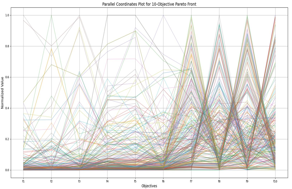
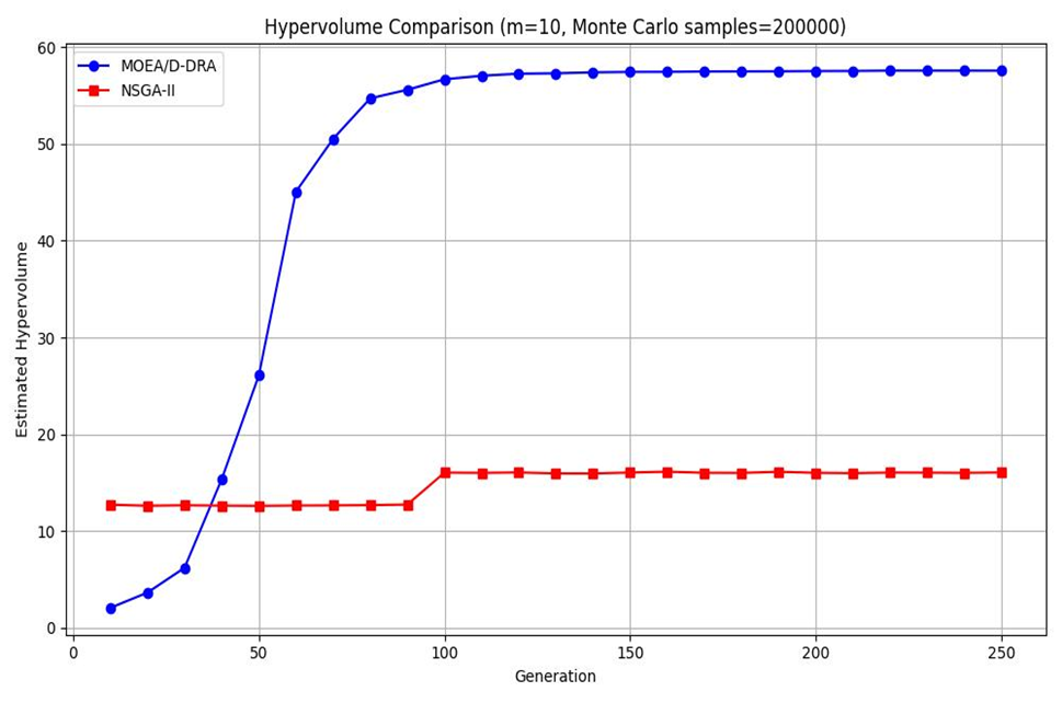
MOEA/D-DRA的超体积逐渐上升,而NSGA-II的超体积却不怎么变化,说明MOEA/D-DRA在高维时对于dtlz1函数具有更好的效果,且MOEA/D-DRA在f1-f5的帕累托前沿的覆盖面更大。
总结
本周主要完成这个高维多目标优化算法。