目录
[1. 图像的灰度直方图](#1. 图像的灰度直方图)
[2. 归一化直方图](#2. 归一化直方图)
[3. 类间方差的定义](#3. 类间方差的定义)
[4. 最优阈值的确定](#4. 最优阈值的确定)
[1. 基本用法](#1. 基本用法)
[2. 参数说明](#2. 参数说明)
[3. 与高斯模糊结合使用](#3. 与高斯模糊结合使用)
[1. 多阈值Otsu's算法](#1. 多阈值Otsu's算法)
[2. 改进的Otsu's算法](#2. 改进的Otsu's算法)
[3. 手动实现Otsu's算法](#3. 手动实现Otsu's算法)
[1. 与全局阈值的对比](#1. 与全局阈值的对比)
[2. 与自适应阈值的对比](#2. 与自适应阈值的对比)
[3. 性能对比](#3. 性能对比)
[1. 硬币检测](#1. 硬币检测)
[2. 文档二值化](#2. 文档二值化)
[3. 细胞计数](#3. 细胞计数)
[1. 图像预处理](#1. 图像预处理)
[2. 直方图分析](#2. 直方图分析)
[3. 阈值类型选择](#3. 阈值类型选择)
[4. 处理复杂图像](#4. 处理复杂图像)
一、Otsu's二值化算法概述
Otsu's二值化算法(大津阈值法)是一种自动阈值选择方法,由日本学者大津展之(Nobuyuki Otsu)于1979年提出。它通过最大化类间方差来确定最优阈值,是图像处理中最常用的阈值分割方法之一。
Otsu's算法的基本思想
Otsu's算法假设图像的直方图是双峰的(即包含前景和背景两个区域),并尝试找到一个阈值T,将图像分为两部分,使得这两部分的类间方差最大。类间方差越大,说明前景和背景的分离效果越好。
Otsu's算法的特点
- 自动化:无需手动设置阈值,算法自动计算最优阈值
- 高效性:计算复杂度低,为O(L),其中L是灰度级数量(通常为256)
- 适应性:适用于直方图呈双峰或多峰分布的图像
- 鲁棒性:对噪声和对比度变化有一定的鲁棒性
二、Otsu's算法的数学原理
1. 图像的灰度直方图
假设图像的灰度级为0到L1(通常L=256),则图像的直方图可以表示为:
H = h0, h1, ..., hL1
其中,hi表示灰度值为i的像素数量。
2. 归一化直方图
归一化直方图表示每个灰度值出现的概率:
p_i = h_i / N
其中,N是图像的总像素数量,满足∑p_i = 1。
3. 类间方差的定义
假设选择阈值T将图像分为两部分:
背景区域:灰度值小于等于T的像素
前景区域:灰度值大于T的像素
(1)概率和
背景像素的总概率:
w0(T) = ∑_{i=0}^T p_i
前景像素的总概率:
w1(T) = ∑_{i=T+1}^{L1} p_i = 1 w0(T)
(2)均值
背景区域的平均灰度值:
μ0(T) = (1 / w0(T)) ∑_{i=0}^T i p_i, 当w0(T) > 0
前景区域的平均灰度值:
μ1(T) = (1 / w1(T)) ∑_{i=T+1}^{L1} i p_i, 当w1(T) > 0
全局平均灰度值:
μ_T = ∑_{i=0}^{L1} i p_i = w0(T) μ0(T) + w1(T) μ1(T)
(3)方差
背景区域的方差:
σ0^2(T) = (1 / w0(T)) ∑_{i=0}^T (i μ0(T))^2 p_i, 当w0(T) > 0
前景区域的方差:
σ1^2(T) = (1 / w1(T)) ∑_{i=T+1}^{L1} (i μ1(T))^2 p_i, 当w1(T) > 0
(4)类间方差
Otsu's算法使用的类间方差定义为:
σ_b^2(T) = w0(T) (μ0(T) μ_T)^2 + w1(T) (μ1(T) μ_T)^2
可以简化为:
σ_b^2(T) = w0(T) w1(T) (μ0(T) μ1(T))^2
4. 最优阈值的确定
Otsu's算法通过遍历所有可能的阈值T(0到L1),找到使类间方差σ_b^2(T)最大的阈值作为最优阈值:
T_opt = argmax_{T=0}^{L1} σ_b^2(T)
三、OpenCV中的Otsu's实现
在OpenCV中,Otsu's二值化算法可以通过cv2.threshold()函数实现,只需在type参数中添加cv2.THRESH_OTSU标志即可。
1. 基本用法
//python
python
import cv2

import numpy as np

from matplotlib import pyplot as plt

 #读取灰度图像

img = cv2.imread('coins.jpg', 0)

 #应用Otsu's阈值分割

ret, thresh = cv2.threshold(img, 0, 255, cv2.THRESH_BINARY_INV + cv2.THRESH_OTSU)

 #显示结果

plt.figure(figsize=(12, 6))

plt.subplot(121), plt.imshow(img, cmap='gray'), plt.title('Original Image')

plt.subplot(122), plt.imshow(thresh, cmap='gray'), plt.title(f'Otsu's Thresholding (T={ret})')

plt.tight_layout()

plt.show()
2. 参数说明
//python
ret, dst = cv2.threshold(src, thresh, maxval, type)
参数说明:
src:输入图像(必须是灰度图像)
thresh:手动设定的阈值(当使用Otsu's算法时,该值会被忽略,通常设为0)
maxval:当像素值超过阈值(或小于阈值,根据type而定)时,赋予的新值
type:阈值类型,必须包含cv2.THRESH_OTSU标志,可以与其他阈值类型组合使用
cv2.THRESH_BINARY + cv2.THRESH_OTSU:二值化 + Otsu's
cv2.THRESH_BINARY_INV + cv2.THRESH_OTSU:反向二值化 + Otsu's
cv2.THRESH_TRUNC + cv2.THRESH_OTSU:截断 + Otsu's(不常用)
cv2.THRESH_TOZERO + cv2.THRESH_OTSU:化零 + Otsu's(不常用)
返回值:
ret:Otsu's算法计算得到的最优阈值
dst:阈值分割后的图像
3. 与高斯模糊结合使用
当图像噪声较大时,Otsu's算法的性能会下降。此时,可以先对图像进行高斯模糊处理,再应用Otsu's阈值分割:
//python
python
import cv2

import numpy as np

from matplotlib import pyplot as plt

 #读取灰度图像

img = cv2.imread('noisy_image.jpg', 0)

 #直接应用Otsu's阈值分割

ret1, thresh1 = cv2.threshold(img, 0, 255, cv2.THRESH_BINARY_INV + cv2.THRESH_OTSU)

 #先高斯模糊,再应用Otsu's阈值分割

blurred = cv2.GaussianBlur(img, (5, 5), 0)

ret2, thresh2 = cv2.threshold(blurred, 0, 255, cv2.THRESH_BINARY_INV + cv2.THRESH_OTSU)

#显示结果

plt.figure(figsize=(15, 10))

plt.subplot(221), plt.imshow(img, cmap='gray'), plt.title('Original Noisy Image')

plt.subplot(222), plt.imshow(thresh1, cmap='gray'), plt.title(f'Otsu's (T={ret1})')

plt.subplot(223), plt.imshow(blurred, cmap='gray'), plt.title('Gaussian Blurred')

plt.subplot(224), plt.imshow(thresh2, cmap='gray'), plt.title(f'Blur + Otsu's (T={ret2})')

plt.tight_layout()

plt.show()

 #显示直方图

plt.figure(figsize=(15, 5))

plt.subplot(121)

plt.hist(img.ravel(), 256, [0, 256])

plt.axvline(x=ret1, color='r', linestyle='', label=f'Otsu's T: {ret1}')

plt.title('Histogram of Original Image')

plt.legend()

plt.subplot(122)

plt.hist(blurred.ravel(), 256, [0, 256])

plt.axvline(x=ret2, color='r', linestyle='', label=f'Otsu's T: {ret2}')

plt.title('Histogram of Blurred Image')

plt.legend()

plt.tight_layout()

plt.show()
四、Otsu's算法的优化与扩展
1. 多阈值Otsu's算法
基本的Otsu's算法只适用于二值分割(前景/背景),但可以扩展到多阈值分割。多阈值Otsu's算法通过最大化类间方差,将图像分割为多个区域。
在OpenCV中,可以使用cv2.ximgproc.threshold模块中的cv2.ximgproc.thresholdOtsu函数实现多阈值分割:
//python
python
import cv2

import numpy as np

from matplotlib import pyplot as plt

 #读取灰度图像

img = cv2.imread('multi_peak_image.jpg', 0)

 #应用单阈值Otsu's算法

ret1, thresh1 = cv2.threshold(img, 0, 255, cv2.THRESH_BINARY + cv2.THRESH_OTSU)

 #应用双阈值Otsu's算法

 注意:需要OpenCV 3.4+版本,并且安装了扩展模块

 可以通过pip install opencvcontribpython安装

thresh2 = cv2.ximgproc.thresholdOtsu(img, k=2)   k=2表示双阈值

 #显示结果

plt.figure(figsize=(15, 8))

plt.subplot(131), plt.imshow(img, cmap='gray'), plt.title('Original Image')

plt.subplot(132), plt.imshow(thresh1, cmap='gray'), plt.title(f'Single Threshold (T={ret1})')

plt.subplot(133), plt.imshow(thresh2, cmap='gray'), plt.title('Dual Threshold')

plt.tight_layout()

plt.show()
2. 改进的Otsu's算法
针对Otsu's算法在处理直方图非双峰分布图像时的局限性,研究者提出了多种改进方法:
(1)基于局部信息的Otsu's算法
结合图像的局部信息(如邻域像素的灰度值),提高Otsu's算法对非均匀光照图像的适应性。
(2)基于遗传算法的Otsu's优化
使用遗传算法搜索最优阈值,提高算法在处理复杂图像时的性能。
(3)快速Otsu's算法
通过减少计算量,提高Otsu's算法的执行速度,适用于实时图像处理场景。
3. 手动实现Otsu's算法
为了更好地理解Otsu's算法的工作原理,我们可以手动实现该算法:
//python
python
import cv2

import numpy as np

from matplotlib import pyplot as plt

def otsu_threshold(image):

     计算图像直方图

    hist, bins = np.histogram(image.ravel(), 256, [0, 256])

     计算归一化直方图

    total_pixels = image.shape[0]  image.shape[1]

    prob = hist / total_pixels

     初始化最大类间方差和最优阈值

    max_variance = 0

    optimal_threshold = 0

     遍历所有可能的阈值(0到255)

    for t in range(256):

         计算背景和前景的概率

        w0 = np.sum(prob[:t+1])

        w1 = 1  w0

        if w0 == 0 or w1 == 0:

            continue

         计算背景和前景的平均灰度值

        mu0 = np.sum(np.arange(t+1)  prob[:t+1]) / w0

        mu1 = np.sum(np.arange(t+1, 256)  prob[t+1:]) / w1

         计算类间方差

        variance = w0  w1  (mu0  mu1)  2


         更新最大类间方差和最优阈值

        if variance > max_variance:

            max_variance = variance

            optimal_threshold = t


    return optimal_threshold


 #读取灰度图像

img = cv2.imread('coins.jpg', 0)

 #使用自定义Otsu's算法

custom_thresh = otsu_threshold(img)

print(f'Custom Otsu\'s threshold: {custom_thresh}')

 #使用OpenCV内置Otsu's算法

ret, thresh_opencv = cv2.threshold(img, 0, 255, cv2.THRESH_BINARY_INV + cv2.THRESH_OTSU)

print(f'OpenCV Otsu\'s threshold: {ret}')


 #应用自定义阈值

ret_custom, thresh_custom = cv2.threshold(img, custom_thresh, 255, cv2.THRESH_BINARY_INV)


 #显示结果

plt.figure(figsize=(15, 6))


plt.subplot(131), plt.imshow(img, cmap='gray'), plt.title('Original Image')

plt.subplot(132), plt.imshow(thresh_custom, cmap='gray'), plt.title(f'Custom Otsu\'s (T={custom_thresh})')

plt.subplot(133), plt.imshow(thresh_opencv, cmap='gray'), plt.title(f'OpenCV Otsu\'s (T={ret})')


plt.tight_layout()

plt.show()
五、Otsu's算法与其他阈值方法的对比
1. 与全局阈值的对比
//python
python
import cv2

import numpy as np

from matplotlib import pyplot as plt

 #读取灰度图像

img = cv2.imread('coins.jpg', 0)

 #全局阈值(手动设置)

ret1, thresh1 = cv2.threshold(img, 130, 255, cv2.THRESH_BINARY_INV)

 #Otsu's阈值

ret2, thresh2 = cv2.threshold(img, 0, 255, cv2.THRESH_BINARY_INV + cv2.THRESH_OTSU)

 #显示结果

plt.figure(figsize=(15, 6))

plt.subplot(131), plt.imshow(img, cmap='gray'), plt.title('Original Image')

plt.subplot(132), plt.imshow(thresh1, cmap='gray'), plt.title(f'Global Threshold (T=130)')

plt.subplot(133), plt.imshow(thresh2, cmap='gray'), plt.title(f'Otsu\'s Threshold (T={ret2})')

plt.tight_layout()

plt.show()
2. 与自适应阈值的对比
//python
python
import cv2
import numpy as np
from matplotlib import pyplot as plt
#读取灰度图像
img = cv2.imread('uneven_lighting.jpg', 0)
#Otsu's阈值
ret1, thresh1 = cv2.threshold(img, 0, 255, cv2.THRESH_BINARY + cv2.THRESH_OTSU)
#自适应阈值(均值法)
thresh2 = cv2.adaptiveThreshold(img, 255, cv2.ADAPTIVE_THRESH_MEAN_C,
cv2.THRESH_BINARY, 11, 2)
#自适应阈值(高斯法)
thresh3 = cv2.adaptiveThreshold(img, 255, cv2.ADAPTIVE_THRESH_GAUSSIAN_C,
cv2.THRESH_BINARY, 11, 2)
#显示结果
plt.figure(figsize=(15, 10))
plt.subplot(221), plt.imshow(img, cmap='gray'), plt.title('Original Image')
plt.subplot(222), plt.imshow(thresh1, cmap='gray'), plt.title(f'Otsu\'s Threshold (T={ret1})')
plt.subplot(223), plt.imshow(thresh2, cmap='gray'), plt.title('Adaptive Mean Threshold')
plt.subplot(224), plt.imshow(thresh3, cmap='gray'), plt.title('Adaptive Gaussian Threshold')
plt.tight_layout()
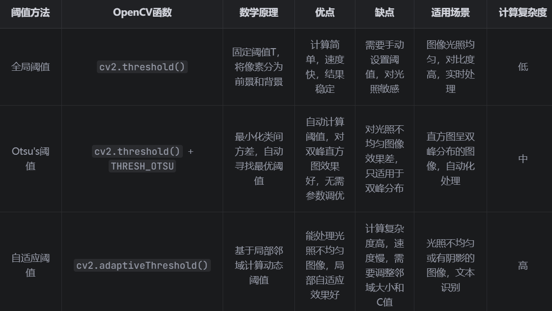
plt.show()3. 性能对比
六、实际应用案例
1. 硬币检测
//python
python
import cv2

import numpy as np

from matplotlib import pyplot as plt

 #读取图像

img = cv2.imread('coins.jpg')

 #转换为灰度图像

gray = cv2.cvtColor(img, cv2.COLOR_BGR2GRAY)

 #高斯模糊

blurred = cv2.GaussianBlur(gray, (11, 11), 0)

 #Otsu's阈值分割

ret, thresh = cv2.threshold(blurred, 0, 255, cv2.THRESH_BINARY_INV + cv2.THRESH_OTSU)

 #形态学操作,去除噪声

kernel = np.ones((3, 3), np.uint8)

opening = cv2.morphologyEx(thresh, cv2.MORPH_OPEN, kernel, iterations=2)

 #检测轮廓

contours, hierarchy = cv2.findContours(opening.copy(), cv2.RETR_EXTERNAL, cv2.CHAIN_APPROX_SIMPLE)

 #绘制轮廓

img_contours = img.copy()

cv2.drawContours(img_contours, contours, 1, (0, 255, 0), 2)

 #显示结果

plt.figure(figsize=(15, 10))

plt.subplot(231), plt.imshow(cv2.cvtColor(img, cv2.COLOR_BGR2RGB)), plt.title('Original Image')

plt.subplot(232), plt.imshow(gray, cmap='gray'), plt.title('Grayscale')

plt.subplot(233), plt.imshow(blurred, cmap='gray'), plt.title('Gaussian Blur')

plt.subplot(234), plt.imshow(thresh, cmap='gray'), plt.title(f'Otsu\'s Threshold (T={ret})')

plt.subplot(235), plt.imshow(opening, cmap='gray'), plt.title('Morphological Opening')

plt.subplot(236), plt.imshow(cv2.cvtColor(img_contours, cv2.COLOR_BGR2RGB)), plt.title(f'Coins Detected: {len(contours)}')

plt.tight_layout()

plt.show()
2. 文档二值化
//python
python
import cv2

import numpy as np

from matplotlib import pyplot as plt

 #读取文档图像

img = cv2.imread('document.jpg')

 #转换为灰度图像

gray = cv2.cvtColor(img, cv2.COLOR_BGR2GRAY)

 #高斯模糊

blurred = cv2.GaussianBlur(gray, (5, 5), 0)

 #Otsu's阈值分割

ret, thresh_otsu = cv2.threshold(blurred, 0, 255, cv2.THRESH_BINARY + cv2.THRESH_OTSU)

 #自适应阈值分割

thresh_adaptive = cv2.adaptiveThreshold(blurred, 255, cv2.ADAPTIVE_THRESH_GAUSSIAN_C,

                                      cv2.THRESH_BINARY, 11, 2)

 #显示结果

plt.figure(figsize=(15, 8))

plt.subplot(221), plt.imshow(cv2.cvtColor(img, cv2.COLOR_BGR2RGB)), plt.title('Original Document')

plt.subplot(222), plt.imshow(gray, cmap='gray'), plt.title('Grayscale')

plt.subplot(223), plt.imshow(thresh_otsu, cmap='gray'), plt.title(f'Otsu\'s Threshold (T={ret})')

plt.subplot(224), plt.imshow(thresh_adaptive, cmap='gray'), plt.title('Adaptive Threshold')

plt.tight_layout()

plt.show()
3. 细胞计数
//python
python
import cv2

import numpy as np

from matplotlib import pyplot as plt

 #读取细胞图像

img = cv2.imread('cells.jpg')

 #转换为灰度图像

gray = cv2.cvtColor(img, cv2.COLOR_BGR2GRAY)

 #高斯模糊

blurred = cv2.GaussianBlur(gray, (7, 7), 0)

 #Otsu's阈值分割

ret, thresh = cv2.threshold(blurred, 0, 255, cv2.THRESH_BINARY_INV + cv2.THRESH_OTSU)

 #形态学操作

kernel = np.ones((5, 5), np.uint8)

closing = cv2.morphologyEx(thresh, cv2.MORPH_CLOSE, kernel, iterations=2)

opening = cv2.morphologyEx(closing, cv2.MORPH_OPEN, kernel, iterations=1)

 #检测轮廓

contours, hierarchy = cv2.findContours(opening.copy(), cv2.RETR_EXTERNAL, cv2.CHAIN_APPROX_SIMPLE)

 #过滤掉小轮廓(噪声)

filtered_contours = []

for contour in contours:

    if cv2.contourArea(contour) > 100:   #调整阈值以过滤不同大小的噪声

        filtered_contours.append(contour)


 #绘制轮廓

img_contours = img.copy()

cv2.drawContours(img_contours, filtered_contours, 1, (0, 255, 0), 2)

 #在轮廓上标注数字

for i, contour in enumerate(filtered_contours):

     计算轮廓的中心坐标

    M = cv2.moments(contour)

    if M["m00"] != 0:

        cx = int(M["m10"] / M["m00"])

        cy = int(M["m01"] / M["m00"])

         #绘制数字

        cv2.putText(img_contours, str(i+1), (cx10, cy+10), cv2.FONT_HERSHEY_SIMPLEX, 0.5, (0, 0, 255), 2)

 #显示结果

plt.figure(figsize=(15, 10))

plt.subplot(231), plt.imshow(cv2.cvtColor(img, cv2.COLOR_BGR2RGB)), plt.title('Original Image')

plt.subplot(232), plt.imshow(gray, cmap='gray'), plt.title('Grayscale')

plt.subplot(233), plt.imshow(blurred, cmap='gray'), plt.title('Gaussian Blur')

plt.subplot(234), plt.imshow(thresh, cmap='gray'), plt.title(f'Otsu\'s Threshold (T={ret})')

plt.subplot(235), plt.imshow(opening, cmap='gray'), plt.title('Morphological Operations')

plt.subplot(236), plt.imshow(cv2.cvtColor(img_contours, cv2.COLOR_BGR2RGB)), plt.title(f'Cells Counted: {len(filtered_contours)}')

plt.tight_layout()

plt.show()

print(f"检测到的细胞数量: {len(filtered_contours)}")
七、注意事项与技巧
1. 图像预处理
- 灰度转换:Otsu's算法只适用于灰度图像,需要先将彩色图像转换为灰度图像
- 噪声处理:使用高斯模糊(cv2.GaussianBlur())减少图像噪声,提高Otsu's算法的性能
- 对比度增强:使用直方图均衡化(cv2.equalizeHist())增强图像对比度,使直方图更容易呈现双峰分布
//python
图像预处理示例
python
import cv2

import numpy as np

from matplotlib import pyplot as plt

 #读取彩色图像

img = cv2.imread('low_contrast.jpg')

 #转换为灰度图像

gray = cv2.cvtColor(img, cv2.COLOR_BGR2GRAY)

 #对比度增强

equalized = cv2.equalizeHist(gray)

 #高斯模糊

blurred = cv2.GaussianBlur(equalized, (5, 5), 0)

 #Otsu's阈值分割

ret, thresh = cv2.threshold(blurred, 0, 255, cv2.THRESH_BINARY_INV + cv2.THRESH_OTSU)

 #显示结果

plt.figure(figsize=(15, 10))

plt.subplot(231), plt.imshow(cv2.cvtColor(img, cv2.COLOR_BGR2RGB)), plt.title('Original Image')

plt.subplot(232), plt.imshow(gray, cmap='gray'), plt.title('Grayscale')

plt.subplot(233), plt.imshow(equalized, cmap='gray'), plt.title('Histogram Equalization')

plt.subplot(234), plt.imshow(blurred, cmap='gray'), plt.title('Gaussian Blur')

plt.subplot(235), plt.imshow(thresh, cmap='gray'), plt.title(f'Otsu\'s Threshold (T={ret})')

 #显示直方图

plt.subplot(236)

plt.hist(blurred.ravel(), 256, [0, 256])

plt.axvline(x=ret, color='r', linestyle='', label=f'Otsu\'s T: {ret}')

plt.title('Histogram')

plt.legend()

plt.tight_layout()

plt.show()
2. 直方图分析
直方图形状:Otsu's算法对双峰直方图效果最好,如果直方图不是双峰的,可以尝试使用图像预处理技术使其呈现双峰分布
阈值位置:观察直方图中Otsu's阈值的位置,确保它位于两个峰值之间
3. 阈值类型选择
目标为白色,背景为黑色:使用cv2.THRESH_BINARY + cv2.THRESH_OTSU
目标为黑色,背景为白色:使用cv2.THRESH_BINARY_INV + cv2.THRESH_OTSU
4. 处理复杂图像
多阈值分割:对于复杂图像,可以使用多阈值Otsu's算法
局部Otsu's:对于光照不均匀的图像,可以将图像分成多个小块,对每个小块应用Otsu's算法
//python
局部Otsu's示例
python
import cv2

import numpy as np

from matplotlib import pyplot as plt

def local_otsu(image, block_size):

    #局部Otsu's阈值分割

    height, width = image.shape

    result = np.zeros_like(image)

     #扩展图像边界,避免边缘处理问题

    pad = block_size // 2

    padded = cv2.copyMakeBorder(image, pad, pad, pad, pad, cv2.BORDER_REFLECT)

     #对每个像素应用局部Otsu's

    for i in range(height):

        for j in range(width):

             #提取局部区域

            block = padded[i:i+block_size, j:j+block_size]

             #计算局部Otsu's阈值

            ret, _ = cv2.threshold(block, 0, 255, cv2.THRESH_BINARY + cv2.THRESH_OTSU)

             #应用阈值

            result[i, j] = 255 if image[i, j] > ret else 0

    return result

 #读取灰度图像

img = cv2.imread('uneven_lighting.jpg', 0)

 #全局Otsu's

ret, thresh_global = cv2.threshold(img, 0, 255, cv2.THRESH_BINARY + cv2.THRESH_OTSU)

 #局部Otsu's

thresh_local = local_otsu(img, block_size=15)

 #显示结果

plt.figure(figsize=(15, 8))

plt.subplot(131), plt.imshow(img, cmap='gray'), plt.title('Original Image')

plt.subplot(132), plt.imshow(thresh_global, cmap='gray'), plt.title(f'Global Otsu\'s (T={ret})')

plt.subplot(133), plt.imshow(thresh_local, cmap='gray'), plt.title('Local Otsu\'s (Block Size=15)')

plt.tight_layout()

plt.show()
八、总结
Otsu's二值化算法是一种经典的自动阈值选择方法,通过最大化类间方差来确定最优阈值。它具有自动化、高效性和适应性等优点,广泛应用于图像处理的各个领域。
主要内容回顾
Otsu's算法原理:基于类间方差最大化,自动选择最优阈值
数学推导:详细介绍了Otsu's算法的数学原理和推导过程
OpenCV实现:使用cv2.threshold()函数,添加cv2.THRESH_OTSU标志启用
优化与扩展:多阈值Otsu's算法、自定义实现和局部Otsu's算法
对比分析:与全局阈值和自适应阈值的对比
实际应用:硬币检测、文档二值化和细胞计数
注意事项:图像预处理、直方图分析和阈值类型选择
使用建议
- 当图像直方图呈双峰分布时,优先选择Otsu's算法
- 对噪声较大的图像,先进行高斯模糊处理
- 对光照不均匀的图像,可以尝试局部Otsu's算法或自适应阈值
- 对于复杂图像,可以结合形态学操作进一步优化分割结果
Otsu's二值化算法是图像处理中的基础技术,掌握它对于理解和应用更复杂的图像处理算法至关重要。通过合理使用Otsu's算法,可以在各种应用场景中获得良好的图像分割效果。