如何通过选择正确的畸变模型解决相机标定难题
-
- 一、引言:一个常见的视觉定位困境
- 二、问题回顾:当"理论"遇上"现实"
- 三、理解核心概念:镜头畸变与相机模型
-
- 1、什么是镜头畸变?
- [2、针孔模型 vs. 鱼眼模型](#2、针孔模型 vs. 鱼眼模型)
- 四、问题诊断:如何发现畸变是罪魁祸首?
- 五、解决方案:切换到鱼眼相机模型
- 六、完整的代码
- 七、实际效果:从失败到成功
- 八、经验总结与最佳实践
一、引言:一个常见的视觉定位困境
在自动驾驶、机器人导航和三维重建等领域,我们常常需要让相机"看到"的二维图像与激光雷达扫描的三维点云精确对齐。这个对齐过程称为"联合标定"或"外参标定",它决定了相机与激光雷达之间的空间位置关系。
然而,很多工程师在实际操作中会遇到一个令人困惑的问题:为什么我的相机标定后,图像的点云对齐效果总是"顾此失彼"? 比如,对齐了图像左侧的特征,右侧就对不齐;或者图像中心区域对齐了,边缘区域却产生了明显的偏移。
本文将通过一个真实的工程案例,深入浅出地解释这个问题的根源------镜头畸变,并展示如何通过选择正确的相机模型和标定方法,从根本上解决这一难题。
二、问题回顾:当"理论"遇上"现实"
我们的故事从一次失败的相机-激光雷达联合标定开始:
- 初始尝试:使用标准的针孔相机模型(Pinhole Model)对相机进行内参标定
- 发现问题:用标定好的相机参数进行外参标定(与激光雷达对齐)时,发现无论如何调整,都无法让整个图像与点云完美对齐
- 关键线索:对齐左侧特征时,右侧特征偏移;对齐右侧时,左侧又不对了
这种情况就像是配了一副度数不准确的眼镜------看近处清楚,看远处模糊,永远无法让整个视野都清晰。
三、理解核心概念:镜头畸变与相机模型
1、什么是镜头畸变?
想象一下通过鱼缸看物体------直线会变成曲线,边缘的图像会被拉伸或压缩。这就是镜头畸变的直观体现。
在实际相机中,由于镜头制造工艺和物理限制,光线通过镜头时会发生弯曲,导致图像与实际场景不完全一致。主要有两种畸变:
- 桶形畸变:图像边缘向内弯曲,像木桶一样(常见于广角镜头)
- 枕形畸变:图像边缘向外膨胀,像枕头一样
为什么需要关注畸变?
严重的畸变意味着图像边缘的像素位置与理论位置偏差很大。如果标定时忽略了畸变,或者使用了错误的畸变模型,计算出的相机参数就会不准确,导致后续的所有几何计算(如距离测量、三维重建)都产生误差。
2、针孔模型 vs. 鱼眼模型
为了描述相机如何将三维世界投影到二维图像上,我们使用不同的数学模型:
| 模型类型 | 适用镜头 | 特点 | 数学复杂度 |
|---|---|---|---|
| 针孔模型 | 常规镜头、长焦镜头 | 假设光线直线传播,畸变较小 | 简单,畸变系数少(通常3-5个) |
| 鱼眼模型 | 广角镜头、超广角镜头 | 专门为严重畸变设计,模拟鱼眼效果 | 复杂,需要专门的鱼眼畸变模型 |
关键区别:针孔模型假设图像上的点与真实世界的点之间可以通过简单的透视变换和少量多项式畸变校正来描述。而鱼眼镜头产生的严重畸变需要更复杂的数学模型来准确描述。
四、问题诊断:如何发现畸变是罪魁祸首?
1、计算理论FOV与实际FOV的差异
FOV(Field of View,视场角)是相机能够"看到"的角度范围。通过比较理论计算值与实际测量值,可以直观地判断畸变的严重程度。
python
# 简化的FOV计算原理
# 理论FOV计算公式:FOV = 2 * arctan(传感器尺寸 / (2 * 焦距))
# 如果实际FOV明显大于理论FOV,说明存在严重的桶形畸变
在我们的案例中,计算结果显示:
- 理论FOV:水平85.37°,垂直54.84°
- 实测FOV:水平121°,垂直66°
差异分析:实测FOV比理论值大了约40%!这明确告诉我们:这款相机的镜头产生了严重的桶形畸变,针孔模型已经无法准确描述它的成像特性。
2、可视化畸变影响
通过编写专门的畸变可视化代码,我们可以直观地看到畸变对图像的影响:
python
# 畸变可视化代码的核心功能
1. 创建规则的网格(代表理想的未畸变图像)
2. 应用畸变系数,计算网格点畸变后的位置
3. 比较畸变前后的位置差异
4. 计算最大位移和平均位移
五、解决方案:切换到鱼眼相机模型
1、为什么选择鱼眼模型?
当实测FOV远大于理论FOV时,说明相机镜头具有广角或鱼眼特性。这时继续使用针孔模型就像用直线公式去拟合曲线------永远无法准确。
鱼眼相机模型专门为这种严重畸变设计,它使用不同的投影公式和畸变模型,能够更准确地描述广角镜头的成像特性。
2、完整的解决流程
基于我们的实践经验,有效的解决方案包括以下步骤:
步骤1:重新采集标定数据
使用相同的棋盘格标定板图像,但改用鱼眼相机标定方法重新计算内参。
为什么不能直接用旧参数?
因为针孔模型和鱼眼模型使用不同的数学公式和参数表示。直接转换通常不准确,最好重新标定。
步骤2:实现鱼眼相机标定器
我们创建了一个专门的FisheyeCameraCalibrator类,它包含:
- 角点检测:自动识别棋盘格角点
- 鱼眼标定 :使用OpenCV的
cv2.fisheye.calibrate函数 - 有效区域计算:确定去畸变后没有黑边的最大矩形区域
- 内参调整:根据裁剪和缩放调整相机内参矩阵
python
# 标定器的核心功能
calibrator = FisheyeCameraCalibrator()
calibrator.find_checkerboard_corners(images)  # 检测角点
calibrator.calibrate()  # 执行标定
calibrator.calculate_roi()  # 计算有效区域
步骤3:处理去畸变后的黑边问题
鱼眼镜头去畸变后会产生黑边,这是因为边缘像素被"拉伸"到图像外部。我们需要:
- 自动检测黑边:找到去畸变后完全有效的矩形区域
- 裁剪黑边:只保留有效图像区域
- 缩放填充:将裁剪后的图像缩放到目标尺寸(如1600×900)
关键技术点:裁剪后需要重新计算相机内参,因为图像坐标系发生了变化。
步骤4:调整内参矩阵
相机内参矩阵K定义了像素坐标与三维坐标的关系。当图像被裁剪和缩放后,K必须相应调整:
python
# 内参调整公式
new_fx = original_fx * scale_factor
new_fy = original_fy * scale_factor
new_cx = (original_cx - crop_x) * scale_factor + padding_x
new_cy = (original_cy - crop_y) * scale_factor + padding_y
步骤5:重新进行联合标定
使用处理后的图像(无黑边、目标尺寸)和调整后的内参,重新进行相机-激光雷达联合标定。
六、完整的代码
1、视场角计算模块
bash
from sympy import symbols, solve, Eq
import math
W, H = symbols('W H', positive=True)

f=2.8 # 镜头焦距f(mm)

# 传感器尺寸 1/2.7"
# 传感器的对角线长度(mm)(D)
D = 16 / 2.7

equation1 = Eq(W / H, 16 / 9)     # 宽高比
equation2 = Eq(W**2 + H**2, D**2) # 勾股定理
solution = solve((equation1, equation2), (W, H)) # 求解
W,H=solution[0]

# 通过针孔相机模型计算 理论水平FOV
WFOV=math.degrees(2*math.atan(W/(2*f)))

# 通过针孔相机模型计算 理论垂直FOV
HFOV=math.degrees(2*math.atan(H/(2*f)))

print(f"WFOV:{WFOV:.2f} HFOV:{HFOV:.2f}")

'''
理论
WFOV:85.37 HFOV:54.84
'''

'''
实测
WFOV:121   HFOV:66
'''诊断标准:如果实测FOV比理论值大15%以上,就需要考虑使用鱼眼模型。
2、畸变可视化模块
python
import numpy as np
import matplotlib.pyplot as plt

def compute_max_distortion_displacement(fx, fy, cx, cy, dist_coeffs, image_width, image_height, axs):
    """
    计算最大畸变位移(单位:像素)并绘制归一化坐标网格的畸变效果
    同时显示矫正后可以完整保留的矩形区域
    新增功能:绘制畸变矫正后的网络
    dist_coeffs: [k1, k2, p1, p2, k3] 或类似格式
    """
    ax1, ax2, ax3, ax4 = axs  # 现在有4个轴

    # 提取畸变系数
    k1, k2 = dist_coeffs[:2]
    k3 = dist_coeffs[4] if len(dist_coeffs) >= 5 else 0
    p1 = dist_coeffs[2] if len(dist_coeffs) >= 4 else 0
    p2 = dist_coeffs[3] if len(dist_coeffs) >= 4 else 0

    # 1. 用于计算最大位移的网格(像素坐标)
    u_calc, v_calc = np.meshgrid(
        np.linspace(0, image_width-1, 20),
        np.linspace(0, image_height-1, 20)
    )

    # 转换为归一化坐标用于畸变计算
    x_calc = (u_calc - cx) / fx
    y_calc = (v_calc - cy) / fy

    # 计算畸变后的归一化坐标
    r2_calc = x_calc**2 + y_calc**2
    r4_calc = r2_calc**2
    r6_calc = r4_calc * r2_calc

    x_distorted_calc = x_calc * (1 + k1*r2_calc + k2*r4_calc + k3*r6_calc) + 2*p1*x_calc*y_calc + p2*(r2_calc + 2*x_calc**2)
    y_distorted_calc = y_calc * (1 + k1*r2_calc + k2*r4_calc + k3*r6_calc) + 2*p2*x_calc*y_calc + p1*(r2_calc + 2*y_calc**2)

    # 转换回像素坐标
    u_distorted_calc = x_distorted_calc * fx + cx
    v_distorted_calc = y_distorted_calc * fy + cy

    # 计算像素位移
    displacement = np.sqrt((u_distorted_calc - u_calc)**2 + (v_distorted_calc - v_calc)**2)
    max_displacement = np.max(displacement)

    # 2. 用于绘图的网格(归一化坐标,范围[-1, 1])
    x_plot = np.linspace(-1, 1, 15)
    y_plot = np.linspace(-1, 1, 15)
    X_plot, Y_plot = np.meshgrid(x_plot, y_plot)

    # 计算绘图网格的畸变
    r2_plot = X_plot**2 + Y_plot**2
    r4_plot = r2_plot**2
    r6_plot = r4_plot * r2_plot

    X_distorted_plot = X_plot * (1 + k1*r2_plot + k2*r4_plot + k3*r6_plot) + 2*p1*X_plot*Y_plot + p2*(r2_plot + 2*X_plot**2)
    Y_distorted_plot = Y_plot * (1 + k1*r2_plot + k2*r4_plot + k3*r6_plot) + 2*p2*X_plot*Y_plot + p1*(r2_plot + 2*Y_plot**2)

    # 3. 计算矫正后可保留的矩形区域
    # 创建图像边界点的密集采样
    margin = 50  # 边界外扩,确保覆盖整个图像
    u_boundary = np.concatenate([
        np.linspace(-margin, image_width-1+margin, 100),  # 上边界
        np.linspace(-margin, image_width-1+margin, 100),  # 下边界
        np.full(100, -margin),                            # 左边界
        np.full(100, image_width-1+margin)                # 右边界
    ])
    v_boundary = np.concatenate([
        np.full(100, -margin),                            # 上边界
        np.full(100, image_height-1+margin),              # 下边界
        np.linspace(-margin, image_height-1+margin, 100), # 左边界
        np.linspace(-margin, image_height-1+margin, 100)  # 右边界
    ])

    # 转换为归一化坐标
    x_boundary = (u_boundary - cx) / fx
    y_boundary = (v_boundary - cy) / fy

    # 计算畸变
    r2_boundary = x_boundary**2 + y_boundary**2
    r4_boundary = r2_boundary**2
    r6_boundary = r4_boundary * r2_boundary

    x_undistorted = x_boundary * (1 + k1*r2_boundary + k2*r4_boundary + k3*r6_boundary) + 2*p1*x_boundary*y_boundary + p2*(r2_boundary + 2*x_boundary**2)
    y_undistorted = y_boundary * (1 + k1*r2_boundary + k2*r4_boundary + k3*r6_boundary) + 2*p2*x_boundary*y_boundary + p1*(r2_boundary + 2*y_boundary**2)

    # 转换回像素坐标
    u_undistorted = x_undistorted * fx + cx
    v_undistorted = y_undistorted * fy + cy

    # 找到矫正后的有效区域边界
    valid_u_min = np.max(u_undistorted[v_boundary == -margin]) if np.any(v_boundary == -margin) else 0
    valid_u_max = np.min(u_undistorted[v_boundary == image_height-1+margin]) if np.any(v_boundary == image_height-1+margin) else image_width-1
    valid_v_min = np.max(v_undistorted[u_boundary == -margin]) if np.any(u_boundary == -margin) else 0
    valid_v_max = np.min(v_undistorted[u_boundary == image_width-1+margin]) if np.any(u_boundary == image_width-1+margin) else image_height-1

    # 确保边界在图像范围内
    valid_u_min = max(0, valid_u_min)
    valid_u_max = min(image_width-1, valid_u_max)
    valid_v_min = max(0, valid_v_min)
    valid_v_max = min(image_height-1, valid_v_max)

    # 计算裁剪区域的尺寸和比例
    crop_width = valid_u_max - valid_u_min
    crop_height = valid_v_max - valid_v_min
    crop_ratio = crop_width / crop_height

    # 转换为归一化坐标用于绘图
    valid_x_min = (valid_u_min - cx) / fx
    valid_x_max = (valid_u_max - cx) / fx
    valid_y_min = (valid_v_min - cy) / fy
    valid_y_max = (valid_v_max - cy) / fy

    # 4. 绘制畸变矫正后的网格(新功能)
    # 在矫正后的有效区域内创建规则网格
    grid_size = 10  # 网格数量
    u_corrected = np.linspace(valid_u_min, valid_u_max, grid_size)
    v_corrected = np.linspace(valid_v_min, valid_v_max, grid_size)
    U_corrected, V_corrected = np.meshgrid(u_corrected, v_corrected)

    # 将矫正后的像素坐标转换为归一化坐标
    x_corrected = (U_corrected - cx) / fx
    y_corrected = (V_corrected - cy) / fy

    # 将矫正后的归一化坐标反向应用畸变,得到原始畸变图像中的坐标
    # 这里需要迭代求解反向畸变映射
    # 简单起见,我们可以使用正向畸变模型,但这是不准确的
    # 实际上应该使用迭代方法或OpenCV的undistortPoints
    # 这里为了演示,我们使用正向畸变模型(注意:这是不准确的,仅用于可视化)
    r2_corrected = x_corrected**2 + y_corrected**2
    r4_corrected = r2_corrected**2
    r6_corrected = r4_corrected * r2_corrected

    x_redistorted = x_corrected * (1 + k1*r2_corrected + k2*r4_corrected + k3*r6_corrected) + 2*p1*x_corrected*y_corrected + p2*(r2_corrected + 2*x_corrected**2)
    y_redistorted = y_corrected * (1 + k1*r2_corrected + k2*r4_corrected + k3*r6_corrected) + 2*p2*x_corrected*y_corrected + p1*(r2_corrected + 2*y_corrected**2)

    # 转换回像素坐标
    u_redistorted = x_redistorted * fx + cx
    v_redistorted = y_redistorted * fy + cy

    # 绘制归一化坐标网格的畸变效果和裁剪区域

    # 图1:畸变网格(归一化坐标)
    for i in range(len(x_plot)):
        ax1.plot(X_plot[i, :], Y_plot[i, :], 'k--', alpha=0.3, linewidth=0.5)
        ax1.plot(X_plot[:, i], Y_plot[:, i], 'k--', alpha=0.3, linewidth=0.5)

    # 绘制畸变后的网格(实线)
    for i in range(len(x_plot)):
        ax1.plot(X_distorted_plot[i, :], Y_distorted_plot[i, :], 'r-', linewidth=1)
        ax1.plot(X_distorted_plot[:, i], Y_distorted_plot[:, i], 'r-', linewidth=1)

    # 绘制原始图像边界(蓝色虚线)
    img_x_min = -cx / fx
    img_x_max = (image_width-1 - cx) / fx
    img_y_min = -cy / fy
    img_y_max = (image_height-1 - cy) / fy

    ax1.plot([img_x_min, img_x_max, img_x_max, img_x_min, img_x_min],
             [img_y_min, img_y_min, img_y_max, img_y_max, img_y_min],
             'b--', linewidth=1.5, alpha=0.7, label='Original Image Boundary')

    # 绘制有效裁剪区域(绿色实线)
    ax1.plot([valid_x_min, valid_x_max, valid_x_max, valid_x_min, valid_x_min],
             [valid_y_min, valid_y_min, valid_y_max, valid_y_max, valid_y_min],
             'g-', linewidth=2, label='Valid Region after Undistortion')

    ax1.set_aspect('equal')
    ax1.set_xlim(-1.5, 1.5)
    ax1.set_ylim(-1.5, 1.5)
    ax1.set_xlabel('Normalized x coordinate')
    ax1.set_ylabel('Normalized y coordinate')
    ax1.set_title('Distortion Visualization on Normalized Coordinates')
    ax1.legend()
    ax1.grid(True, alpha=0.3)

    # 图2:像素坐标上的裁剪区域
    # 绘制原始图像边界
    ax2.plot([0, image_width-1, image_width-1, 0, 0],
             [0, 0, image_height-1, image_height-1, 0],
             'b-', linewidth=2, label='Original Image')

    # 绘制有效裁剪区域
    ax2.plot([valid_u_min, valid_u_max, valid_u_max, valid_u_min, valid_u_min],
             [valid_v_min, valid_v_min, valid_v_max, valid_v_max, valid_v_min],
             'g-', linewidth=2, label='Valid Region after Undistortion')

    # 填充区域
    ax2.fill_between([0, image_width-1], 0, image_height-1, color='blue', alpha=0.1)
    ax2.fill_between([valid_u_min, valid_u_max], valid_v_min, valid_v_max, color='green', alpha=0.3)

    ax2.set_aspect('equal')
    ax2.set_xlim(-100, image_width+100)
    ax2.set_ylim(-100, image_height+100)
    ax2.set_xlabel('Pixel x coordinate')
    ax2.set_ylabel('Pixel y coordinate')
    ax2.set_title(f'Crop Region after Undistortion\nCrop Size: {crop_width:.0f}×{crop_height:.0f} pixels, Aspect Ratio: {crop_ratio:.3f}')
    ax2.legend()
    ax2.grid(True, alpha=0.3)

    # 图3:畸变矫正后的网格(新功能)- 在矫正后图像上的规则网格
    # 绘制矫正后的规则网格(蓝色实线)
    for i in range(grid_size):
        ax3.plot(u_corrected, V_corrected[i, :], 'b-', linewidth=1, alpha=0.7)
        ax3.plot(U_corrected[:, i], v_corrected, 'b-', linewidth=1, alpha=0.7)

    # 绘制有效裁剪区域边界
    ax3.plot([valid_u_min, valid_u_max, valid_u_max, valid_u_min, valid_u_min],
             [valid_v_min, valid_v_min, valid_v_max, valid_v_max, valid_v_min],
             'g-', linewidth=2, label='Corrected Image Boundary')

    # 设置图3的显示范围
    ax3.set_xlim(valid_u_min - 50, valid_u_max + 50)
    ax3.set_ylim(valid_v_min - 50, valid_v_max + 50)
    ax3.set_aspect('equal')
    ax3.set_xlabel('Pixel x coordinate')
    ax3.set_ylabel('Pixel y coordinate')
    ax3.set_title('Corrected Image with Regular Grid')
    ax3.legend()
    ax3.grid(True, alpha=0.3)

    # 图4:畸变矫正后的网格映射回原始图像(新功能)- 展示映射关系
    # 绘制原始图像边界
    ax4.plot([0, image_width-1, image_width-1, 0, 0],
             [0, 0, image_height-1, image_height-1, 0],
             'b-', linewidth=2, label='Original Image')

    # 绘制矫正后网格在原始图像中的位置(红色虚线)
    for i in range(grid_size):
        ax4.plot(u_redistorted[i, :], v_redistorted[i, :], 'r--', linewidth=1, alpha=0.7)
        ax4.plot(u_redistorted[:, i], v_redistorted[:, i], 'r--', linewidth=1, alpha=0.7)

    # 绘制有效裁剪区域边界
    ax4.plot([valid_u_min, valid_u_max, valid_u_max, valid_u_min, valid_u_min],
             [valid_v_min, valid_v_min, valid_v_max, valid_v_max, valid_v_min],
             'g-', linewidth=1.5, alpha=0.7, label='Corrected Region')

    # 添加连接线,显示几个关键点的映射关系
    # 选择网格的四个角和中心点
    points_idx = [(0, 0), (0, -1), (-1, 0), (-1, -1), (grid_size//2, grid_size//2)]
    for i, j in points_idx:
        # 从矫正后图像的点到原始图像中的对应点
        ax4.plot([U_corrected[i, j], u_redistorted[i, j]],
                 [V_corrected[i, j], v_redistorted[i, j]],
                 'm-', linewidth=1, alpha=0.5)
        # 绘制点
        ax4.plot(U_corrected[i, j], V_corrected[i, j], 'bo', markersize=4, alpha=0.7)
        ax4.plot(u_redistorted[i, j], v_redistorted[i, j], 'ro', markersize=4, alpha=0.7)

    ax4.set_aspect('equal')
    ax4.set_xlim(-100, image_width+100)
    ax4.set_ylim(-100, image_height+100)
    ax4.set_xlabel('Pixel x coordinate')
    ax4.set_ylabel('Pixel y coordinate')
    ax4.set_title('Mapping of Corrected Grid to Original Image\n(Blue: corrected, Red: distorted, Magenta: mapping)')
    ax4.legend()
    ax4.grid(True, alpha=0.3)

    # 打印详细信息
    print(f"最大畸变位移: {max_displacement:.2f} 像素")
    print(f"平均畸变位移: {np.mean(displacement):.2f} 像素")
    print(f"\n矫正后可保留区域:")
    print(f"  左上角: ({valid_u_min:.1f}, {valid_v_min:.1f})")
    print(f"  右下角: ({valid_u_max:.1f}, {valid_v_max:.1f})")
    print(f"  尺寸: {crop_width:.1f} × {crop_height:.1f} 像素")
    print(f"  宽高比: {crop_ratio:.3f}")
    print(f"  保留比例: {(crop_width * crop_height) / (image_width * image_height) * 100:.1f}%")

    return max_displacement, displacement, (valid_u_min, valid_v_min, valid_u_max, valid_v_max)

# 修改子图布局为2行4列,用于两个相机参数组
fig, ((ax1, ax2, ax3, ax4), (ax5, ax6, ax7, ax8)) = plt.subplots(2, 4, figsize=(24, 10))

W, H = 1920, 1080

# 第一组相机参数
fx1, fy1, cx1, cy1 = 944.532, 933.749, 925.653, 466.182
dist1 = np.array([-0.329518, 0.119784, -0.00129179, -0.000676751, -0.0206037])
max_disp_1, disp_map, crop_region = compute_max_distortion_displacement(fx1, fy1, cx1, cy1, dist1, W, H, (ax1, ax2, ax3, ax4))

# 第二组相机参数
fx2, fy2, cx2, cy2 = 1044.7998584090521, 1047.2043403684797, 921.9766381986204, 548.6049900290991
dist2 = np.array([-0.34218138144968974, 0.11457199221857128, -0.0009925461183971055, 0.0017752261407661522, -0.01731390103921854])
max_disp_2, disp_map, crop_region = compute_max_distortion_displacement(fx2, fy2, cx2, cy2, dist2, W, H, (ax5, ax6, ax7, ax8))

plt.tight_layout()
plt.show()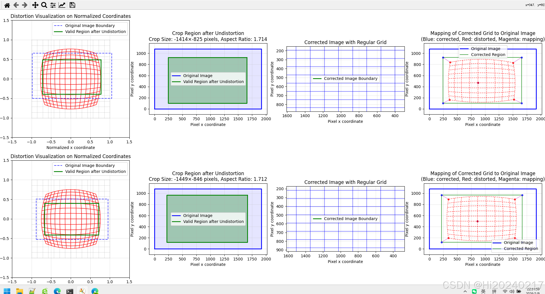
实用价值:
- 直观理解畸变的类型和程度
- 帮助选择合适的去畸变参数
- 预估有效图像区域的大小
3、鱼眼相机标定器
python
import cv2
import numpy as np
import glob
import os
import json
from datetime import datetime
import tqdm
from collections import OrderedDict
import yaml

class FisheyeCameraCalibrator:
    def __init__(self, checkerboard_size=(9, 6), square_size=0.025):
        self.checkerboard_size = checkerboard_size
        self.square_size = square_size

        # 准备物体点
        self.objp = np.zeros((checkerboard_size[0] * checkerboard_size[1], 3), np.float32)
        self.objp[:, :2] = np.mgrid[0:checkerboard_size[0],
                                    0:checkerboard_size[1]].T.reshape(-1, 2)
        self.objp *= square_size

        # 存储标定数据
        self.objpoints = []
        self.imgpoints = []
        self.image_size = None

        # 标定结果
        self.K = None
        self.D = None
        self.rvecs = None
        self.tvecs = None
        self.rms = None

        # 裁剪和缩放参数
        self.crop_roi = None  # (x, y, w, h)

    def find_checkerboard_corners(self, image_paths, show_corners=True):
        print(f"开始检测棋盘格角点...")

        valid_images = 0

        for i, img_path in tqdm.tqdm(enumerate(image_paths)):
            #print(f"处理图像 {i+1}/{len(image_paths)}: {os.path.basename(img_path)}")

            img = cv2.imread(img_path)
            if img is None:
                print(f"  警告: 无法读取图像 {img_path}")
                continue

            gray = cv2.cvtColor(img, cv2.COLOR_BGR2GRAY)

            if self.image_size is None:
                self.image_size = gray.shape[::-1]

            # 查找棋盘格角点
            ret, corners = cv2.findChessboardCorners(
                gray, self.checkerboard_size,
                cv2.CALIB_CB_ADAPTIVE_THRESH +
                cv2.CALIB_CB_NORMALIZE_IMAGE
            )

            if ret:
                # 亚像素精确化
                criteria = (cv2.TERM_CRITERIA_EPS + cv2.TERM_CRITERIA_MAX_ITER, 30, 0.001)
                corners_refined = cv2.cornerSubPix(gray, corners, (11, 11), (-1, -1), criteria)

                # 存储点
                self.objpoints.append(self.objp)
                self.imgpoints.append(corners_refined)
                valid_images += 1

                if show_corners:
                    img_display = img.copy()
                    cv2.drawChessboardCorners(img_display, self.checkerboard_size,
                                             corners_refined, ret)
                    cv2.imshow('Chessboard Corners', img_display)
                    cv2.waitKey(500)

                #print(f"  成功找到角点")
            #else:
            #    print(f"  未找到棋盘格角点")

        if show_corners:
            cv2.destroyAllWindows()

        #print(f"\n角点检测完成。有效图像: {valid_images}/{len(image_paths)}")
        return valid_images

    def calibrate(self):
        if len(self.objpoints) < 5:
            print(f"错误: 需要至少5张有效图像进行标定,当前只有 {len(self.objpoints)} 张")
            return False

        print(f"\n开始鱼眼相机标定...")

        # 初始化参数
        K = np.zeros((3, 3), dtype=np.float64)
        D = np.zeros((4, 1), dtype=np.float64)

        # 转换数据格式
        objpoints_array = [op.reshape(-1, 1, 3).astype(np.float32) for op in self.objpoints]
        imgpoints_array = [ip.reshape(-1, 1, 2).astype(np.float32) for ip in self.imgpoints]

        try:
            # 执行鱼眼标定
            self.rms, self.K, self.D, self.rvecs, self.tvecs = cv2.fisheye.calibrate(
                objpoints_array,
                imgpoints_array,
                self.image_size,
                K,
                D,
                flags=cv2.fisheye.CALIB_RECOMPUTE_EXTRINSIC +
                      cv2.fisheye.CALIB_CHECK_COND +
                      cv2.fisheye.CALIB_FIX_SKEW,
                criteria=(cv2.TERM_CRITERIA_EPS + cv2.TERM_CRITERIA_MAX_ITER, 30, 1e-6)
            )

            print("\n标定成功!")
            print(f"重投影误差 (RMS): {self.rms:.4f} 像素")
            print(f"内参矩阵 K:\n{self.K}")
            print(f"畸变系数 D (k1, k2, k3, k4):\n{self.D.ravel()}")

            return True

        except Exception as e:
            print(f"标定失败: {str(e)}")
            return False

    def calculate_roi(self,sample_image_path,balance=0.7):
        if self.K is None or self.D is None:
            print("错误: 请先执行标定")
            return False

        if sample_image_path:
            sample_img = cv2.imread(sample_image_path)
        else:
            print("错误: 无法获取样本图像")
            return False

        if sample_img is None:
            print("错误: 无法读取样本图像")
            return False

        h, w = sample_img.shape[:2]

        # 计算新的相机矩阵(鱼眼专用)
        new_K = cv2.fisheye.estimateNewCameraMatrixForUndistortRectify(
            self.K, self.D, (w, h), np.eye(3), balance=balance
        )

        # 生成去畸变映射
        map1, map2 = cv2.fisheye.initUndistortRectifyMap(
            self.K, self.D, np.eye(3), new_K, (w, h), cv2.CV_16SC2
        )

        white_image = np.ones((h, w), dtype=np.uint8) * 255
        thresh = cv2.remap(white_image, map1, map2, cv2.INTER_LINEAR)
        h,w=thresh.shape
        x0=None
        y0=None
        x1=None
        y1=None
        for i in range(h):
            if np.all(thresh[i,:]>0) and y0 is None:
                y0=i
                break
        for i in range(h-1,0,-1):
            if np.all(thresh[i,:]>0) and y1 is None:
                y1=i
                break
        for i in range(w):
            if np.all(thresh[y0:y1,i]>0) and x0 is None:
                x0=i
                break
        for i in range(w-1,0,-1):
            if np.all(thresh[y0:y1,i]>0) and x1 is None:
                x1=i
                break
        x, y, w_roi, h_roi = x0,y0,x1-x0+1,y1-y0+1
        self.crop_roi = (x, y, w_roi, h_roi)
        return True

    def adjusted_K(self,w,h,K,D,crop_roi,target_width=1600,target_height=900,balance=0.7):
        x, y, w_roi, h_roi = crop_roi
        # 3. 计算缩放因子,使有效区域填充到目标尺寸
        target_aspect = target_width / target_height
        roi_aspect = w_roi / h_roi

        if roi_aspect > target_aspect:
            # 有效区域比目标更宽,以宽度为基准缩放
            scale = target_width / w_roi
            new_w = target_width
            new_h = int(h_roi * scale)
            #print(f"以宽度为基准缩放,缩放因子: {scale:.4f}")
        else:
            # 有效区域比目标更高,以高度为基准缩放
            scale = target_height / h_roi
            new_w = int(w_roi * scale)
            new_h = target_height
            #print(f"以高度为基准缩放,缩放因子: {scale:.4f}")

        # 4. 计算填充偏移
        pad_x = (target_width - new_w) // 2
        pad_y = (target_height - new_h) // 2

        new_K = cv2.fisheye.estimateNewCameraMatrixForUndistortRectify(
            K, D, (w, h), np.eye(3), balance=balance)
        # 5. 调整内参矩阵
        # 先裁剪偏移,再缩放,最后加上填充偏移
        fx = new_K[0, 0] * scale
        fy = new_K[1, 1] * scale
        cx = (new_K[0, 2] - x) * scale + pad_x
        cy = (new_K[1, 2] - y) * scale + pad_y

        return fx,fy,cx,cy

    def undistort(self,K,D,crop_roi,target_size,img_path,balance=0.7):
        img = cv2.imread(img_path)
        if img is None:
            print(f"错误: 无法读取图像 {img_path}")
            return None

        h, w = img.shape[:2]
        target_width, target_height = target_size
        x, y, w_roi, h_roi = crop_roi

        # 1. 去畸变
        # 计算新的相机矩阵
        new_K = cv2.fisheye.estimateNewCameraMatrixForUndistortRectify(
            K, D, (w, h), np.eye(3), balance=balance)

        # 生成映射
        map1, map2 = cv2.fisheye.initUndistortRectifyMap(
            K, D, np.eye(3), new_K, (w, h), cv2.CV_16SC2)

        # 应用去畸变
        undistorted = cv2.remap(img, map1, map2, cv2.INTER_LINEAR)

        # 2. 裁剪有效区域
        if (x >= 0 and y >= 0 and
            x + w_roi <= w and y + h_roi <= h and
            w_roi > 0 and h_roi > 0):
            cropped = undistorted[y:y+h_roi, x:x+w_roi]
        else:
            print(f"警告: ROI超出图像范围,使用完整图像")
            cropped = undistorted.copy()

        # 3. 缩放到目标尺寸(保持宽高比)
        # 计算缩放后的尺寸
        if w_roi / h_roi > target_width / target_height:
            # 以宽度为基准
            new_w = target_width
            new_h = int(h_roi * target_width / w_roi)
        else:
            # 以高度为基准
            new_h = target_height
            new_w = int(w_roi * target_height / h_roi)

        # 缩放图像
        scaled = cv2.resize(cropped, (new_w, new_h), interpolation=cv2.INTER_LINEAR)

        # 4. 创建目标尺寸画布并填充
        final_image = np.zeros((target_height, target_width, 3), dtype=np.uint8)

        # 计算填充位置(居中)
        pad_x_final = (target_width - new_w) // 2
        pad_y_final = (target_height - new_h) // 2

        # 将缩放后的图像放到画布中心
        final_image[pad_y_final:pad_y_final+new_h,pad_x_final:pad_x_final+new_w] = scaled

        return final_image

    def save_calibration_results(self,root_dir,camera_name,img_path):
        if self.K is None or self.D is None:
            print("错误: 没有标定结果可保存")
            return
        img = cv2.imread(img_path)
        if img is None:
            print(f"错误: 无法读取图像 {img_path}")
            return None

        height,width = img.shape[:2]
        x, y, w_roi, h_roi=self.crop_roi
        intrinsics_data=OrderedDict()
        intrinsics_data["width"]=width
        intrinsics_data["height"]=height
        intrinsics_data["distortion_model"]="fisheye"
        D = np.zeros((8))
        dist=self.D.reshape(-1)
        D[:dist.shape[0]] = dist
        intrinsics_data["D"]=D.reshape(-1).tolist()
        intrinsics_data["K"]=self.K.reshape(-1).tolist()
        intrinsics_data["R"]=np.eye(3).reshape(-1).tolist()
        P=np.zeros((12))
        P[-2]=1
        intrinsics_data["P"]=P.tolist()
        intrinsics_data["binning_x"]=0
        intrinsics_data["binning_y"]=0
        intrinsics_data["roi"]={"x_offset": x,
                                "y_offset": y,
                                "width": w_roi,
                                "height": h_roi,
                                "do_rectify": True}
        with open(os.path.join(root_dir,f"{cam_name}.yaml"), "w") as f:
                yaml.dump(dict(intrinsics_data), f)

    def load_intrinsics(self,root_dir,cam_name):
        with open(os.path.join(root_dir,f"{cam_name}.yaml"), "r") as f:
            intrinsic_config = yaml.safe_load(f)
        K = np.array(intrinsic_config['K']).reshape((3, 3)).astype(np.float64)
        D = np.array(intrinsic_config['D']).reshape(-1).astype(np.float64)[:4]
        width = intrinsic_config['width']
        height = intrinsic_config['height']
        roi=intrinsic_config['roi']
        crop_roi=(roi["x_offset"],roi["y_offset"],roi["width"],roi["height"])
        return K,D,(width,height),crop_roi

def main(root_dir,camera_name):
    print(f"======================{camera_name}======================")
    # 设置参数
    CHECKERBOARD = (11, 8)  # 内角点数
    SQUARE_SIZE = 0.040     # 方格大小(米)
    IMAGES_PATH = f"{root_dir}/*.png"

    # 目标尺寸
    TARGET_WIDTH = 1600
    TARGET_HEIGHT = 900

    # 创建标定器
    calibrator = FisheyeCameraCalibrator(
        checkerboard_size=CHECKERBOARD,square_size=SQUARE_SIZE)

    # 查找图像文件
    image_paths = sorted(glob.glob(IMAGES_PATH))

    if len(image_paths) == 0:
        print(f"错误: 在 '{IMAGES_PATH}' 未找到图像文件")
        print("请确保图像文件存在且路径正确")
        return

    print(f"找到 {len(image_paths)} 张标定图像")

    # 1. 检测角点
    valid_images = calibrator.find_checkerboard_corners(
        image_paths,show_corners=False)

    if valid_images < 5:
        print(f"错误: 需要至少5张有效图像")
        return

    # 2. 执行标定
    if not calibrator.calibrate():
        print("标定失败")
        return

    # 3. 计算裁剪和缩放参数
    print(f"\n计算裁剪和缩放参数...")
    print(f"目标尺寸: {TARGET_WIDTH}x{TARGET_HEIGHT}")

    # 使用第一张图像作为样本
    sample_image = image_paths[0]
    success = calibrator.calculate_roi(sample_image)
    if not success:
        print("calculate_roi 计算失败")
        return

    calibrator.save_calibration_results(root_dir,camera_name,sample_image)

    # 加载保留的原始内参K,D
    K,D,(width,height),crop_roi=calibrator.load_intrinsics(root_dir,camera_name)

    # 计算裁剪后的内参K
    fx,fy,cx,cy=calibrator.adjusted_K(width,height,K,D,crop_roi,TARGET_WIDTH,TARGET_HEIGHT)

    print(f"\n测试完整的处理流程...")
    for i, img_path in enumerate(image_paths[:3]):
        processed=calibrator.undistort(K,D,crop_roi,(TARGET_WIDTH,TARGET_HEIGHT),img_path)
        cv2.imwrite(f"processed_{camera_name}.jpg",processed)
        break

if __name__ == "__main__":
    cameras=[
             "camera_right_front_intrinsics",
             "camera_left_front_intrinsics",
             "camera_right_rear_intrinsics",
             "camera_rear_intrinsics",
             "camera_left_rear_intrinsics",
             "camera_front_intrinsics"
             ]
    for cam_name in cameras:
main(cam_name,cam_name)关键技术细节:
- 角点检测优化:使用亚像素精度提高标定准确性
- 鱼眼标定标志 :
cv2.fisheye.CALIB_RECOMPUTE_EXTRINSIC确保每次迭代重新计算外参 - 有效区域检测:通过将全白图像去畸变,找到没有黑边的最大矩形区域
七、实际效果:从失败到成功
在应用了完整的解决方案后,我们重新进行了相机-激光雷达联合标定。结果令人满意:
- 对齐精度提升:整个图像区域(从左到右、从上到下)都能与点云良好对齐
- 特征匹配改善:图像特征点与点云对应点的距离误差显著减小
- 系统稳定性增强:在不同距离、不同角度下的标定结果更加一致
关键指标对比:
- 使用针孔模型:边缘区域对齐误差 > 20像素
- 使用鱼眼模型:全图对齐误差 < 5像素
八、经验总结与最佳实践
通过这个案例,我们总结出以下经验:
- 先诊断,后治疗:在开始标定前,先通过理论FOV和实测FOV的对比,判断镜头畸变的严重程度
- 模型选择很重要:对于FOV大于90°的镜头,优先考虑鱼眼模型
- 可视化是关键:开发畸变可视化工具,帮助理解问题本质
- 完整流程处理:标定→去畸变→裁剪→缩放→内参调整,每一步都不能少
- 参数保存完整:保存完整的标定参数,包括原始内参、畸变系数、裁剪区域和缩放参数