一、RANSAC 是解决什么问题的?
👉 在含有大量离群点(Outliers)的数据中,鲁棒地估计模型参数
典型场景
-
特征匹配中 错误匹配很多
-
点云中 噪声 + 伪点
-
拟合直线 / 平面 / 单应矩阵 / 基础矩阵
-
PnP 前的 2D--3D 对应点中有假点
普通最小二乘(LS)的问题:
-
对离群点极其敏感
-
一个坏点就能"拉歪"整个模型
RANSAC 的思想是:
宁可只用一小撮"干净点",也不被脏点污染
宁可只用一小撮"干净点",也不被脏点污染
宁可只用一小撮"干净点",也不被脏点污染
二、RANSAC核心思想
随机抽最小样本 → 拟合模型 → 统计内点 → 重复 → 选内点最多的模型
利用随机采样和一致性检验的方法,来取分数据中的内点和外点,内点是指符合模型的数据,外点是指不符合模型的数据。
三、RANSAC 算法流程(标准版)
设模型参数为 θ
Step 1:随机采样(Minimal Sample Set)
-
随机选 最小数量 的点
-
例如:
-
直线:2 点
-
平面:3 点
-
单应矩阵:4 对点
-
基础矩阵:8 点(8-point)
-
Step 2:模型估计
-
用最小样本估计模型
-
通常是 解析解 / DLT
Step 3:一致性检测(Inlier Test)
- 对所有点计算误差:

Step 4:统计内点数
- 记录内点数量
Step 5:重复 N 次
- 找到 内点最多 的模型
Step 6(可选):模型重估
-
用所有内点
-
再做一次 最小二乘 / LM
📌 RANSAC + LM = 工程黄金搭档
四、RANSAC 数学本质
1️⃣ 目标不是最小误差,而是:

2️⃣ 内点概率驱动迭代次数
若:
-
内点比例:w
-
最小样本数:s
-
成功概率:p
所需迭代次数:

案例一RANSAC 拟合二维直线(最经典)
1️⃣ 构造数据(含离群点)
cpp
clc; clear; close all;

% 真实直线 y = 2x + 1
x_in = linspace(0,10,50);
y_in = 2*x_in + 1 + randn(size(x_in))*0.3;

% 离群点
x_out = rand(1,20)*10;
y_out = rand(1,20)*20;

x = [x_in x_out];
y = [y_in y_out];

figure; hold on; grid on;
scatter(x, y, 'b');
title('原始数据(含离群点)');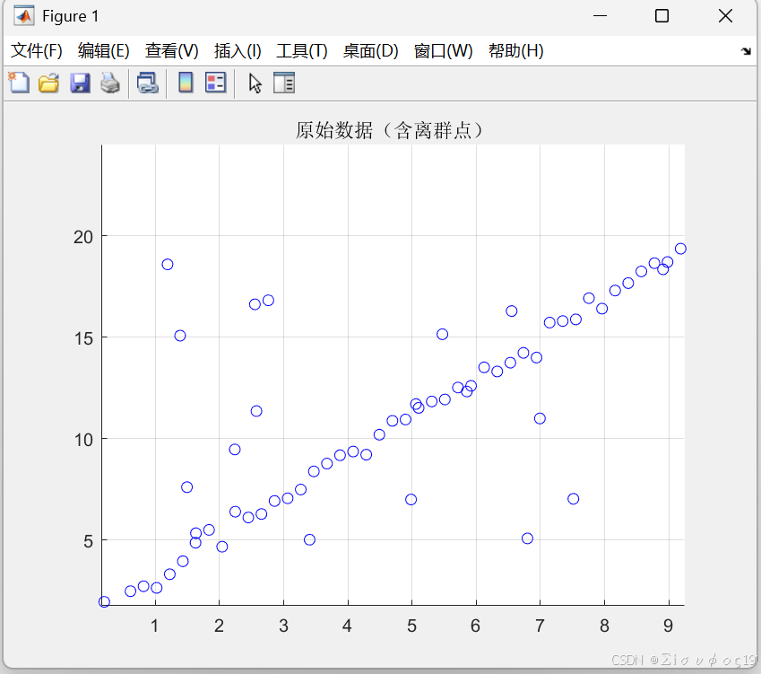
2️⃣ RANSAC 实现
cpp
clc; clear; close all;

% 真实直线 y = 2x + 1     50个直线上的点
x_in = linspace(0,10,50);
y_in = 2*x_in + 1 + randn(size(x_in))*0.3;

% 离群点  20个离群点
x_out = rand(1,20)*10;
y_out = rand(1,20)*20;


% 直线点+离群点=70 个
x = [x_in x_out];
y = [y_in y_out];

figure; hold on; grid on;
scatter(x, y, 'b');
title('原始数据(含离群点)');


% 迭代次数
num_iter = 1000;
% 点到直线的距离阈值判断
threshold = 0.5;


% 把最好的内点集合起来
best_inliers = [];

for i = 1:num_iter
    % 随机选2个点
    idx = randperm(length(x), 2);
    x1 = x(idx(1)); y1 = y(idx(1));
    x2 = x(idx(2)); y2 = y(idx(2));

    % 拟合直线 ax + by + c = 0
    a = y2 - y1;
    b = x1 - x2;
    c = x2*y1 - x1*y2;

    % 计算点到直线距离
    dist = abs(a*x + b*y + c) / sqrt(a^2 + b^2);

    inliers = find(dist < threshold);

    if length(inliers) > length(best_inliers)
        best_inliers = inliers;

    end
end


x_in = x(best_inliers);
y_in = y(best_inliers);

% 拟合
p = polyfit(x_in, y_in, 1);

x_fit = linspace(0,10,100);
y_fit = polyval(p, x_fit);

figure; hold on; grid on;
scatter(x, y, 'b');
scatter(x_in, y_in, 'r');
plot(x_fit, y_fit, 'k', 'LineWidth',2);
legend('All points','Inliers','RANSAC Line');
title('RANSAC 直线拟合结果');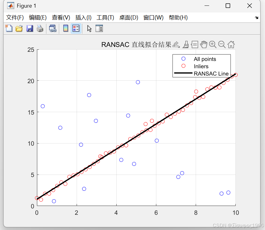
案例二 RANSAC 拟合圆
原理:
1️⃣ 圆的一般方程

2️⃣ 最小样本数(Minimal Sample Set)
👉 3 个不共线点
(这是圆的解析最小解)
3️⃣ 点到圆的误差(RANSAC 判据)
常用误差:

实例
1:构造测试数据(含离群点)
cpp
clc; clear; close all;

% 真实圆参数
a0 = 5; b0 = 4; r0 = 3;

theta = linspace(0,2*pi,80);
x_in = a0 + r0*cos(theta) + randn(size(theta))*0.05;
y_in = b0 + r0*sin(theta) + randn(size(theta))*0.05;

% 离群点
x_out = rand(1,30)*10;
y_out = rand(1,30)*10;

x = [x_in x_out];
y = [y_in y_out];

figure; hold on; axis equal; grid on;
scatter(x, y, 'b');
title('原始数据(含离群点)');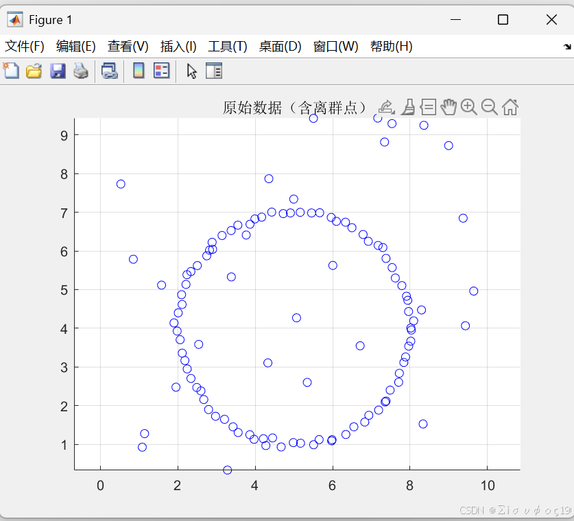
2、RANSAC 拟合圆核心代码
cpp
num_iter = 2000;
threshold = 0.1;

best_inliers = [];
best_circle = [];

N = length(x);

for k = 1:num_iter

    % 随机选 3 个点
    idx = randperm(N,3);
    x1 = x(idx(1)); y1 = y(idx(1));
    x2 = x(idx(2)); y2 = y(idx(2));
    x3 = x(idx(3)); y3 = y(idx(3));

    % 判断是否共线(行列式)
    if abs(det([x1 y1 1; x2 y2 1; x3 y3 1])) < 1e-3
        continue;
    end

    % ===== 解析求圆心和半径 =====
    A = 2*[x2-x1, y2-y1;
           x3-x1, y3-y1];
    B = [x2^2+y2^2 - x1^2-y1^2;
         x3^2+y3^2 - x1^2-y1^2];

    C = A\B;
    a = C(1);
    b = C(2);
    r = sqrt((x1-a)^2 + (y1-b)^2);

    % ===== 计算内点 =====
    dist = abs(sqrt((x-a).^2 + (y-b).^2) - r);
    inliers = find(dist < threshold);

    % 更新最优模型
    if length(inliers) > length(best_inliers)
        best_inliers = inliers;
        best_circle = [a b r];
    end
end
3、用内点进行最小二乘精修(强烈推荐)
cpp
xin = x(best_inliers);
yin = y(best_inliers);

% 代数最小二乘(线性)
A = [2*xin(:), 2*yin(:), ones(length(xin),1)];
B = xin(:).^2 + yin(:).^2;

param = A\B;

a = param(1);
b = param(2);
r = sqrt(param(3) + a^2 + b^2);
4、可视化
cpp
theta = linspace(0,2*pi,200);
xc = a + r*cos(theta);
yc = b + r*sin(theta);

figure; hold on; axis equal; grid on;
scatter(x, y, 'b');
scatter(x(best_inliers), y(best_inliers), 'r');
plot(xc, yc, 'k', 'LineWidth',2);
legend('All points','Inliers','RANSAC Circle');
title('RANSAC 圆拟合结果');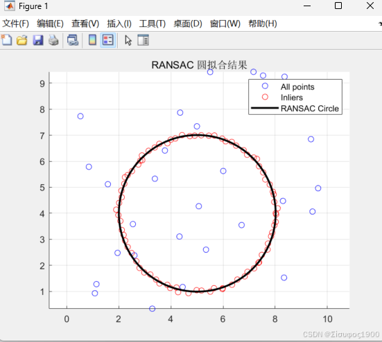
案例三、RANSAC 拟合平面
典型应用:
-
点云地面分割(无人车)
-
工件基准面
-
结构光参考平面
-
ICP / PnP / BA 前的几何约束
平面数学模型
1️⃣ 平面一般式

2️⃣ 最小样本数(Minimal Sample Set)
👉 3 个不共线点
3️⃣ 点到平面距离(RANSAC 判据)

实例:
构造测试点云(含离群点)
cpp
clc; clear; close all;

% 真实平面:z = 0.5x + 0.2y + 1
[xg, yg] = meshgrid(linspace(0,5,20));
zg = 0.5*xg + 0.2*yg + 1 + randn(size(xg))*0.05;

% 转为点集
pts_in = [xg(:), yg(:), zg(:)];

% 离群点
pts_out = rand(80,3)*6;

pts = [pts_in; pts_out];
RANSAC 主循环
cpp
num_iter = 2000;
threshold = 0.1;

best_inliers = [];
best_plane = [];

N = size(pts,1);

for k = 1:num_iter

    % 随机选3点
    idx = randperm(N,3);
    p1 = pts(idx(1),:);
    p2 = pts(idx(2),:);
    p3 = pts(idx(3),:);

    % 共线判断
    v1 = p2 - p1;
    v2 = p3 - p1;
    n = cross(v1,v2);

    if norm(n) < 1e-6
        continue;
    end

    % 平面参数
    n = n / norm(n);
    d = -dot(n,p1);

    % 点到平面距离
    dist = abs(pts*n' + d);

    inliers = find(dist < threshold);

    if length(inliers) > length(best_inliers)
        best_inliers = inliers;
        best_plane = [n d];
    end
end
用内点进行最小二乘精修(SVD)
cpp
in_pts = pts(best_inliers,:);

% 去中心
centroid = mean(in_pts,1);
Q = in_pts - centroid;

% SVD
[~,~,V] = svd(Q,0);
n = V(:,end);
d = -dot(n,centroid);

best_plane = [n' d];
结果可视化
cpp
figure; hold on; grid on; axis equal;
scatter3(pts(:,1),pts(:,2),pts(:,3),'b.');
scatter3(in_pts(:,1),in_pts(:,2),in_pts(:,3),'r.');

% 绘制平面
[xp,yp] = meshgrid(linspace(0,5,10));
zp = -(best_plane(1)*xp + best_plane(2)*yp + best_plane(4)) / best_plane(3);
surf(xp,yp,zp,'FaceAlpha',0.5,'EdgeColor','none');

legend('All points','Inliers','Plane');
title('RANSAC 平面拟合');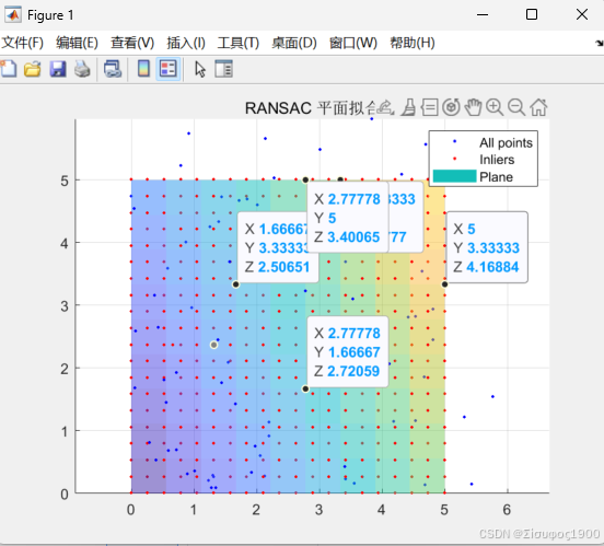
HALCON / PCL 对应参数
cpp
segment_planes_object_model_3d(
    ObjectModel3D,
    'distance_threshold', DistanceThreshold,
    'min_support', MinSupport,
    ObjectModel3DPlanes,
    PlaneInfo
)


pcl::SACSegmentation<pcl::PointXYZ> seg;
seg.setModelType(pcl::SACMODEL_PLANE);
seg.setMethodType(pcl::SAC_RANSAC);
seg.setDistanceThreshold(0.01);
seg.setMaxIterations(1000);
seg.setProbability(0.99);