机器学习入门（十六）集成学习，GBDT，XGBoost

提升树（Boosting Decision Tree ）

• 思想

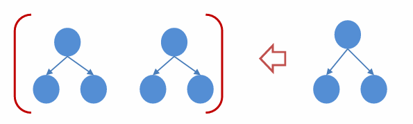
• 通过拟合残差的思想来进行提升

• 残差：真实值 - 预测值

• 生活中的例子

• 预测某人的年龄为100岁

• 第1次预测：对100岁预测，预测成80岁；100 -- 80 = 20（残差）

• 第2次预测：上一轮残差20岁作为目标值，预测成16岁；20 -- 16 = 4 （残差）

• 第3次预测：上一轮的残差4岁作为目标值，预测成3.2岁；4 -- 3.2 = 0.8（残差）

• 若三次预测的结果串联起来： 80 + 16 + 3.2 = 99.2

通过拟合残差可将多个弱学习器组成一个强学习器，这就是提升树的最朴素思想

梯度提升树（Gradient Boosting Decision Tree）

梯度提升树不再拟合残差，而是利用梯度下降的近似方法，利用损失函数的负梯度作为提升树算法中的残差近似值。

假设：

1.前一轮迭代得到的强学习器是：

2.损失函数为平方损失是：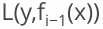

3.本轮迭代的目标是找到一个弱学习器：

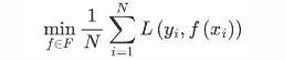
4.让本轮的损失最小化:

5.则要拟合的负梯度为:

GBDT 拟合的负梯度就是残差。如果我们的 GBDT 进行的是分类问题，则损失函数变为 logloss，此时拟合的目标值就是该损失函数的负梯度值

例：

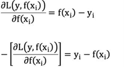
初始化弱学习器(CART树)：

当模型预测值为何值时，会使得第一个弱学习器的平方误差最小，即：求损失函数对 f(𝑥𝑖) 的导数，并令导数为0.

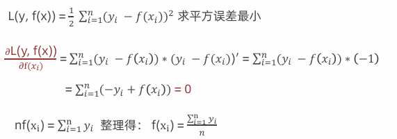
从公式可得：初始化树桩输出值为目标值的均值时，可使得第一个弱学习器的平方误差最小。10个样本，均值:7.31。

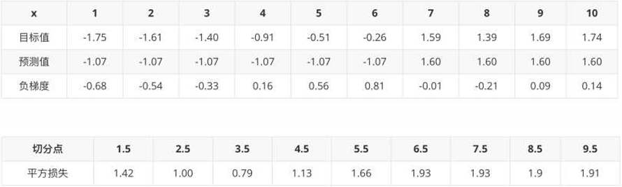
1、构建第1个弱学习器，根据负梯度的计算方法得到下表：

当1.5为切分点：拟合负梯度 5.56 - 7.31 = -1.75, 5.7 - 7.31 = -1.61, -1.40, -0.91, ... , 1.74

左子树：1个样本 -1.75，右子树9个样本：-1.61，-1.40，-0.91...

左子树均值为：- 1.75/1 = -1.75；右子树均值为：((-1.61) + (-1.40)+(-0.91)+(-0.51)+(-0.26)+1.59 +1.39 + 1.69 + 1.74 )/9 = 0.19

计算平方损失：左子树(-1.75+1.75)^2 + 右子树：(-1.61-0.19)^2 + (-1.40-0.19)^2 + (-0.91-0.19)^2 + (-0.51-0.19)^2 +(-0.26-0.19)^2 + (1.59-0.19)^2 + (1.39-0.19)^2 + (1.69-0.19)^2 + (1.74-0.19)^2 = 15.72308

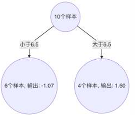
2、当 6.5 作为切分点时，平方损失最小，此时得到第1棵决策树

大于6.5,7~10输出：(1.59 + 1.39 + 1.69 + 1.74）/ 4 = 1.6025

小于6.5,1~6输出：(-1.75 - 1.61 - 1.4 - 0.91 - 0.51 - 0.26) / 6 = -1.07

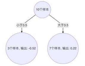
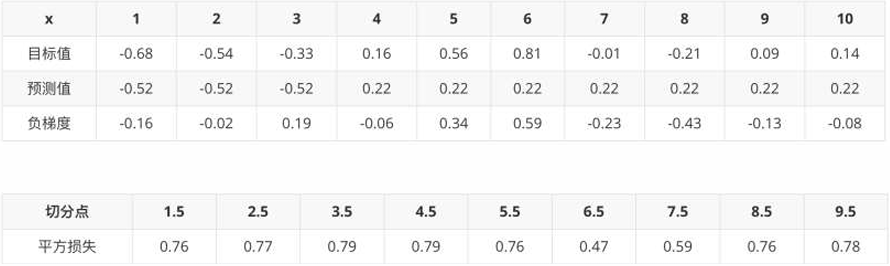
3、构建第2个弱学习器

4、以3.5 作为切分点时，平方损失最小，此时得到第2棵决策树

5、构建第3个弱学习器

6、以6.5 作为切分点时，平方损失最小，此时得到第3棵决策树

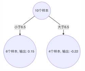
7、构建最终弱学习器

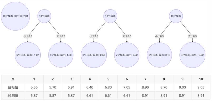
以x=6样本为例：输入到最终学习器中的结果：7.31 + (-1.07) + 0.22 + 0.15 = 6.61

梯度提升树的构建流程

1 初始化弱学习器（目标值的均值作为预测值）

2 迭代构建学习器，每一个学习器拟合上一个学习器的负梯度

3 直到达到指定的学习器个数

4 当输入未知样本时，将所有弱学习器的输出结果组合起来作为强学习器的输出

例一：

python 复制代码

# 1.导入依赖包
import pandas as pd
from sklearn.model_selection import train_test_split, GridSearchCV
from sklearn.tree import DecisionTreeClassifier
from sklearn.ensemble import GradientBoostingClassifier
from sklearn.metrics import accuracy_score


def dm01():
    # 2.读取数据
    taitan_df = pd.read_csv('./data/titanic/train.csv')

    # 3.数据基本处理准备
    # 3.1 获取x y
    x = taitan_df[[
        'Pclass',
        'Age',
        'Sex',
        'SibSp',
        'Parch',
        'Fare',
        'Embarked'
    ]].copy()
    y = taitan_df['Survived'].copy()
    # 3.2 缺失值处理
    x['Age'].fillna(x['Age'].mean(), inplace=True)
    # 3.3 pclass离散型数据需one-hot编码
    x = pd.get_dummies(x)
    # 3.4 数据集划分
    x_train, x_test, y_train, y_test = train_test_split(x, y, random_state=22, test_size=0.2)

    # 4.GBDT 训练和评估
    estimator = GradientBoostingClassifier()
    estimator.fit(x_train, y_train)
    mysorce = estimator.score(x_test, y_test)
    print("gbdt mysorce-->1", mysorce)

    # 5.GBDT 网格搜索交叉验证
    estimator = GradientBoostingClassifier()
    param = {
        "n_estimators": [100, 110, 120, 130],
        "max_depth": [4, 6, 8, 10],
        "random_state": [9]
    }
    estimator = GridSearchCV(estimator, param_grid=param, cv=3)
    estimator.fit(x_train, y_train)
    mysorce = estimator.score(x_test, y_test)
    print("gbdt mysorce-->2", mysorce)
    print(estimator.best_estimator_)


dm01()

执行结果

python 复制代码

gbdt mysorce-->1 0.7988826815642458
gbdt mysorce-->2 0.8268156424581006
GradientBoostingClassifier(max_depth=4, random_state=9)

XGBoost (eXtreme Gradient Boosting)

• 极端梯度提升树，集成学习方法的王牌，在数据挖掘比赛中，大部分获胜者用了XGBoost。

• XGBoost的构建思想：

1、构建模型的方法是最小化训练数据的损失函数

训练的模型复杂度较高，易过拟合。

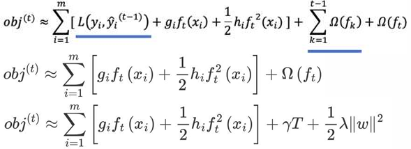
2、在损失函数中加入正则化项

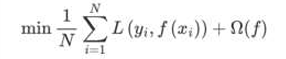
提高对未知的测试数据的泛化性能。

XGBoost（Extreme Gradient Boosting）是对GBDT的改进，并且在损失函数中加入了正则化项

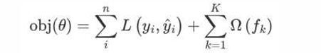
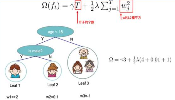
• 正则化项用来降低模型的复杂度

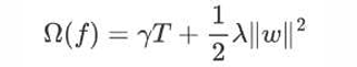
• γT 中的 T 表示一棵树的叶子结点数量。

• λ||w||2中的 w 表示叶子结点输出值组成的向量，||w|| 向量的模；λ对该项的调节系数。

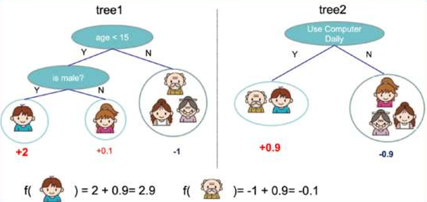
假设我们要预测一家人对电子游戏的喜好程度，考虑到年轻和年老相比，年轻更可能喜欢电子游戏，以及男性和女性相比，男性更喜欢电子游戏，故先根据年龄大小区分小孩和大人，然后再通过性别区分开是男是女，逐一给各人在电子游戏喜好程度上打分：

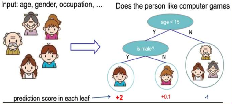
训练出tree1和tree2，类似之前GBDT的原理，两棵树的结论累加起来便是最终的结论

树tree1的复杂度表示为

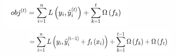
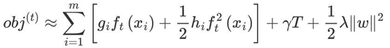
进行t次迭代的学习模型的目标函数如下为：

直接对目标函数求解比较困难，通过泰勒展开将目标函数换一种近似的表示方式

•泰勒展开

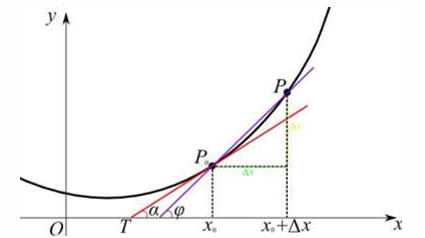
将一个函数在某一点处展开成无限项的多项式表达式

•一阶泰勒展开

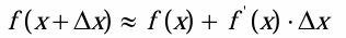
•二阶泰勒展开

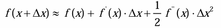
• 目标函数对进行泰勒二阶展开，得到如下近似表示的公式

• 其中gi和 hi的分别为损失函数的一阶导、二阶导：

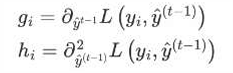
• 观察目标函数，发现以下两项表示t-1个弱学习器构成学习器的目标函数，都是常数，我们可以将其去掉：

从样本角度转为按照叶子节点输出角度，优化损失函数

gi 表示每个样本的一阶导，hi表示每个样本的二阶导
ft(xi) 表示样本的预测值
T 表示叶子结点的数目

4.||w||2 由叶子结点值组成向量的模

举个例子：请计算10样本在叶子结点上的输出表示

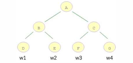
例如：m=10 个样本，落在 D 结点 3 个样本，落在 E 结点 2 个样本，落在 F 结点 2 个样本，落在 G 结点 3 个样本；计算 gi∗ft 𝑥3 的表达形式如下：

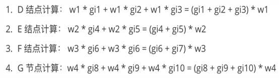
目标函数中的各项可以做以下转换：

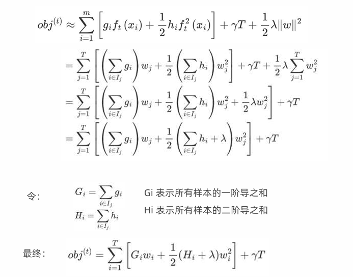
• 求损失函数最小值

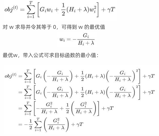
目标函数最终为：

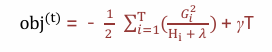
该公式也叫做打分函数 (scoring function)，从损失函数、树的复杂度两个角度来衡量一棵树的优劣。当我们构建树时，可以用来选择树的划分点，具体操作如下式所示：

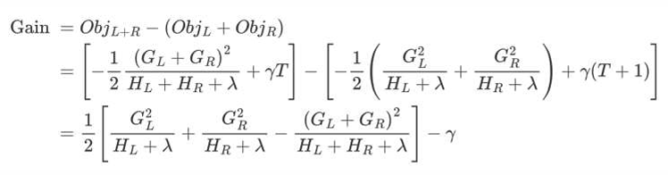
根据上一页PPT中计算的Gain值：

1.对树中的每个叶子结点尝试进行分裂

2.计算分裂前 -分裂后的分数：

如果Gain > 0，则分裂之后树的损失更小，会考虑此次分裂
如果Gain< 0，说明分裂后的分数比分裂前的分数大，此时不建议分裂

3.当触发以下条件时停止分裂：

达到最大深度
叶子结点数量低于某个阈值
所有的结点在分裂不能降低损失
等等..

XGBoost详细数学计算示例

1. 数据集准备

假设我们有4个样本，一个特征值x，对应目标值y：

样本	x	y
1	1	15
2	2	20
3	3	25
4	4	30

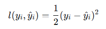
使用平方损失函数：

2. 超参数设置

树的数量：2棵（K=2）
学习率：η = 0.3
正则化参数：λ = 1，γ = 0
每棵树的最大深度：2层
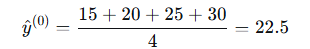
初始预测：所有样本预测为平均值

3. 第一棵树（t=1）的构建

3.1 初始化和梯度计算

初始预测：所有样本预测值为均值

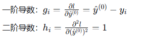
计算一阶导数和二阶导数（对于平方损失函数）：

计算结果：

样本	y	y^(0)	g_i	h_i
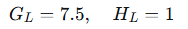
1	15	22.5	7.5	1
2	20	22.5	2.5	1
3	25	22.5	-2.5	1
4	30	22.5	-7.5	1

3.2 寻找第一个分裂点

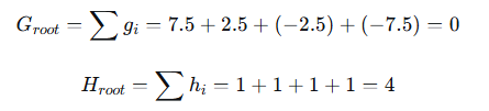
根节点包含所有4个样本。计算根节点的统计量：

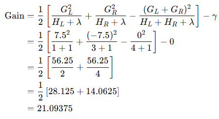
尝试在x=1.5处分裂（介于样本1和2之间）：

左子节点（x≤1.5）：样本1

右子节点（x>1.5）：样本2，3，4

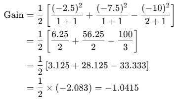
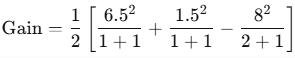
计算增益（Gain）：

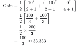
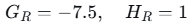
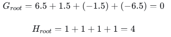
尝试在x=2.5处分裂（介于样本2和3之间）：

左子节点（x≤2.5）：样本1,2
右子节点（x>2.5）：样本3,4

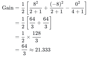
计算增益：

尝试在x=3.5处分裂（介于样本3和4之间）：

左子节点（x≤3.5）：样本1,2,3

右子节点（x>3.5）：样本4

计算增益：

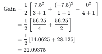
选择最大增益：x=2.5处增益最大（33.333），因此在此处分裂。

3.3 继续分裂左子节点

左子节点包含样本1和2，统计量：

尝试在x=3.5处分裂：

右左节点（x≤3.5）：样本3

右右节点（x>3.5）：样本4

计算增益：

增益为负，不分裂。右子节点成为叶子节点。

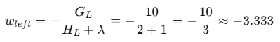
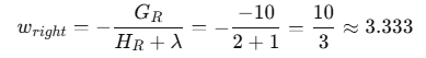
3.5 计算叶子节点权重

现在树结构已确定：根节点在x=2.5处分裂，生成两个叶子节点。

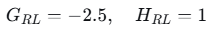
左叶子节点（样本1和2）：

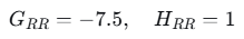
右叶子节点（样本3和4）：

3.6 更新预测值

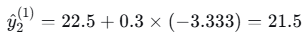
学习率η = 0.3

对于每个样本：

样本1（落入左叶子）：

样本2（落入左叶子）：

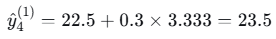
样本3（落入右叶子）：

样本4（落入右叶子）：

4. 第二棵树（t=2）的构建

4.1 计算梯度统计量

基于第一棵树后的预测值：

样本	y	y^(1)y^(1)	g_i = y^(1)−yiy^(1)−yi	h_i = 1
1	15	21.5	6.5	1
2	20	21.5	1.5	1
3	25	23.5	-1.5	1
4	30	23.5	-6.5	1

4.2 寻找第一个分裂点

根节点统计量：

尝试在x=2.5处分裂：

左子节点：样本1,2

右子节点：样本3,4

计算增益：

4.3 继续分裂

左子节点和右子节点的进一步分裂：

1,2左子节点在x=1.5处分裂的增益：

增益为正，继续分裂。

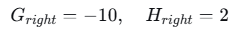
3,4右子节点在x=3.5处分裂的增益：

增益为正，继续分裂。

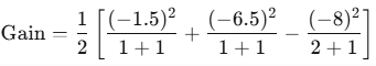
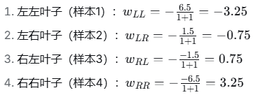
4.4 计算叶子节点权重

最终树结构：根节点在x=2.5处分裂，左子节点在x=1.5处分裂，右子节点在x=3.5处分裂。

四个叶子节点的权重：

4.5 更新最终预测值

学习率η = 0.3

样本1

样本2

样本3

样本4

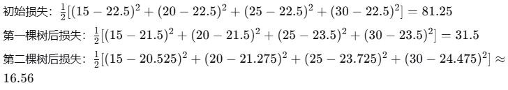
5. 最终结果总结

两棵树后的预测值与真实值对比：

样本	x	真实值y	初始预测	第一棵树后	第二棵树后
1	1	15	22.5	21.5	20.525
2	2	20	22.5	21.5	21.275
3	3	25	22.5	23.5	23.725
4	4	30	22.5	23.5	24.475

损失变化：

例红酒品质分类

已知数据集共包含 11 个特征，共计 3269 条数据. 我们通过训练模型来预测红酒的品质, 品质共有 6个类别，分别使用数字:0、1、2、3、4、5 来表示

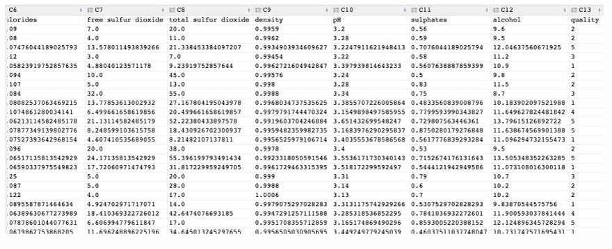
• 需求：对红酒品质进行多分类

• 分析：从数据可知 1、目标是多分类 2、数据存在样本不均衡问题

代码

python 复制代码

# 1.导入依赖包
import joblib
import numpy as np
import pandas as pd
from xgboost import XGBClassifier
from collections import Counter
from sklearn.model_selection import train_test_split
from sklearn.metrics import classification_report
from sklearn.model_selection import StratifiedKFold


def dm01():
    # 2.数据读取及基本数据处理
    # 2.1 加载训练集
    data = pd.read_csv('./data/红酒品质分类.csv')
    # 2.2 数据预处理
    x = data.iloc[:, :-1]
    y = data.iloc[:, -1] - 3
    # 2.3 数据集划分
    x_train, x_test, y_train, y_test = train_test_split(x, y, test_size=0.2, random_state=40)
    # 2.4 数据存储,axis=1按列水平拼接
    pd.concat([x_train, y_train], axis=1).to_csv('data/红酒品质分类-train.csv')
    pd.concat([x_test, y_test], axis=1).to_csv('data/红酒品质分类-test.csv')


def dm02():
    # 2.数据读取及预处理
    # 2.1 加载数据集
    train_data = pd.read_csv('./data/红酒品质分类-train.csv')
    test_data = pd.read_csv('./data/红酒品质分类-test.csv')
    # 2.2 准备数据 训练集测试集
    x_train = train_data.iloc[:, :-1]
    y_train = train_data.iloc[:, -1]
    x_test = test_data.iloc[:, :-1]
    y_test = test_data.iloc[:, -1]
    print(x_train.shape, y_train.shape, x_test.shape, y_test.shape)

    # 3.XGBoost模型训练
    estimator = XGBClassifier(
        n_estimators=100,
        objective='multi: softmax',
        eval_metric='merror',
        eta=0.1,
        # use_label_encoder=False,
        random_state=22,
    )
    estimator.fit(x_train, y_train)

    # 4.XGBoost模型预测及评估
    y_pred = estimator.predict(x_test)
    print(classification_report(y_true=y_test, y_pred=y_pred, zero_division=0))
    print(estimator.score(x_test, y_test))

    # 5.模型保存
    joblib.dump(estimator, './data/mymodelxgboost.pth')


# 1.导入依赖包
from sklearn.utils import class_weight


def dm03():
    # 2.数据读取及数据预处理
    # 2.1 加载数据集
    train_data = pd.read_csv('./data/红酒品质分类-train.csv')
    test_data = pd.read_csv('./data/红酒品质分类-test.csv')
    # 2.2 准备数据 训练集测试集
    x_train = train_data.iloc[:, :-1]
    y_train = train_data.iloc[:, -1]
    x_test = test_data.iloc[:, :-1]
    y_test = test_data.iloc[:, -1]
    print(x_train.shape, y_train.shape, x_test.shape, y_test.shape)
    # 2.3 样本不均衡问题处理
    classes_weights = class_weight.compute_sample_weight(class_weight='balanced', y=y_train)

    # 3.XGBoost模型训练
    estimator = XGBClassifier(
        # n_estimators=150,
        # objective='multi: softmax',
        # eval_metric='merror',
        # eta=0.1,
        # # use_label_encoder=False,
        # random_state=22,
    )
    # 训练的时候，指定样本的权重
    estimator.fit(x_train, y_train, sample_weight=classes_weights)
    # estimator.fit(x_train, y_train)
    # 4.XGBoost模型预测及评估
    y_pred = estimator.predict(x_test)
    print(classification_report(y_true=y_test, y_pred=y_pred, zero_division=0))


# 1.导入依赖包
from sklearn.model_selection import StratifiedKFold
from sklearn.model_selection import GridSearchCV


def dm04():
    # 2.读取数据及数据预处理
    # 2.1 加载数据集
    train_data = pd.read_csv('./data/红酒品质分类-train.csv')
    test_data = pd.read_csv('./data/红酒品质分类-test.csv')

    # 2.2 准备数据 训练集测试集
    x_train = train_data.iloc[:, :-1]
    y_train = train_data.iloc[:, -1]
    x_test = test_data.iloc[:, :-1]
    y_test = test_data.iloc[:, -1]
    print(x_train.shape, y_train.shape, x_test.shape, y_test.shape)
    # 2.3 交叉验证时,采用分层抽取
    spliter = StratifiedKFold(n_splits=5, shuffle=True)

    # 3.模型训练
    # 3.1 定义超参数
    param_grid = {
        'max_depth': np.arange(3, 5, 1),
        'n_estimators': np.arange(50, 150, 50),
        'eta': np.arange(0.1, 1, 0.3)
    }
    # 3.2实例化XGBoost
    estimator = XGBClassifier(
        learning_rate=0.05,
        n_estimators=100,
        objective='multi: softmax',
        eval_metric='merror',
        eta=0.1,
        random_state=22
    )
    # 3.3 实例化cv工具
    estimator = GridSearchCV(
        estimator=estimator,
        param_grid=param_grid,
        cv=spliter
    )
    # 3.4 训练模型
    estimator.fit(x_train, y_train)

    # 4.模型预测及评估
    y_pred = estimator.predict(x_test)
    print(classification_report(y_true=y_test, y_pred=y_pred, zero_division=0))
    print('estimator.best_estimator_ -->', estimator.best_estimator_)
    print('estimator.best_params_ -->', estimator.best_params_)


dm01()
dm02()
dm03()
dm04()

执行结果

复制代码

(1279, 12) (1279,) (320, 12) (320,)
              precision    recall  f1-score   support

           0       0.00      0.00      0.00         3
           1       0.00      0.00      0.00         8
           2       0.77      0.86      0.82       136
           3       0.68      0.74      0.71       125
           4       0.70      0.50      0.58        42
           5       0.00      0.00      0.00         6

    accuracy                           0.72       320
   macro avg       0.36      0.35      0.35       320
weighted avg       0.69      0.72      0.70       320

0.721875
(1279, 12) (1279,) (320, 12) (320,)
              precision    recall  f1-score   support

           0       0.00      0.00      0.00         3
           1       0.00      0.00      0.00         8
           2       0.77      0.79      0.78       136
           3       0.66      0.70      0.68       125
           4       0.58      0.52      0.55        42
           5       0.00      0.00      0.00         6

    accuracy                           0.68       320
   macro avg       0.34      0.34      0.34       320
weighted avg       0.66      0.68      0.67       320

(1279, 12) (1279,) (320, 12) (320,)
              precision    recall  f1-score   support

           0       0.00      0.00      0.00         3
           1       0.00      0.00      0.00         8
           2       0.72      0.83      0.77       136
           3       0.63      0.70      0.66       125
           4       0.60      0.36      0.45        42
           5       0.00      0.00      0.00         6

    accuracy                           0.67       320
   macro avg       0.33      0.31      0.31       320
weighted avg       0.63      0.67      0.65       320

estimator.best_estimator_ --> XGBClassifier(base_score=None, booster=None, callbacks=None,
              colsample_bylevel=None, colsample_bynode=None,
              colsample_bytree=None, device=None, early_stopping_rounds=None,
              enable_categorical=False, eta=0.1, eval_metric='merror',
              feature_types=None, gamma=None, grow_policy=None,
              importance_type=None, interaction_constraints=None,
              learning_rate=0.05, max_bin=None, max_cat_threshold=None,
              max_cat_to_onehot=None, max_delta_step=None, max_depth=4,
              max_leaves=None, min_child_weight=None, missing=nan,
              monotone_constraints=None, multi_strategy=None, n_estimators=100,
              n_jobs=None, num_parallel_tree=None, ...)
estimator.best_params_ --> {'eta': 0.1, 'max_depth': 4, 'n_estimators': 100}

机器学习入门（十六）集成学习，GBDT，XGBoost

提升树 （Boosting Decision Tree ）

梯度提升树 （Gradient Boosting Decision Tree）

例一：

XGBoost (eXtreme Gradient Boosting)

XGBoost详细数学计算示例

1. 数据集准备

2. 超参数设置

3. 第一棵树（t=1）的构建

3.1 初始化和梯度计算

3.2 寻找第一个分裂点

3.3 继续分裂左子节点

3.5 计算叶子节点权重

3.6 更新预测值

4. 第二棵树（t=2）的构建

4.1 计算梯度统计量

4.2 寻找第一个分裂点

4.3 继续分裂

4.4 计算叶子节点权重

4.5 更新最终预测值

5. 最终结果总结

例红酒品质分类

提升树（Boosting Decision Tree ）

梯度提升树（Gradient Boosting Decision Tree）