逻辑回归实战：从原理到不平衡数据优化（含欠拟合/过拟合诊断与召回率提升）

一、什么是逻辑回归？

逻辑回归（Logistic Regression）虽然名字带"回归"，但本质是一个分类算法 ，尤其擅长解决二分类问题（也可扩展至多分类）。

核心思想

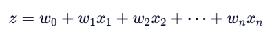
• 通过线性组合输入特征：

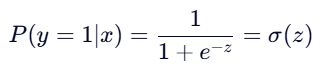
• 将 z 映射到 (0,1) 区间，表示属于正类的概率：

• 决策规则：若 P(y=1∣x)>0.5P(y=1∣x)>0.5 ，则预测为正类（1），否则为负类（0）。

优点 ：模型简单、可解释性强（权重反映特征重要性）、训练高效。
局限：假设特征与对数几率（log-odds）线性相关，对非线性关系建模能力弱。

---

二、如何判断逻辑回归模型好不好？------ 关键评估指标

在不平衡数据中，准确率（Accuracy）是"毒药"！例如欺诈检测中，99.9% 的交易正常，模型全预测"正常"也能获得 99.9% 准确率，但毫无价值。

必看指标（基于混淆矩阵）

指标	意义	适用场景
召回率（Recall）	查全率：有多少正样本被找出来了？	欺诈检测、疾病筛查（宁可误报，不可漏报）
精确率（Precision）	查准率：预测为正的样本中有多少是真的？	垃圾邮件过滤（避免误杀正常邮件）
F1-Score	精确率与召回率的调和平均	综合评估
AUC-ROC	模型在不同阈值下的整体性能	通用，尤其适合不平衡数据

💡 银行老赖检测 ：召回率是核心指标！目标是尽可能找出所有潜在老赖客户（即使误报一些正常交易）。

---

三、模型诊断：欠拟合 vs 过拟合

1. 欠拟合（Underfitting）

• 表现：训练集和测试集性能都很差（如 Recall < 0.5）
• 原因 ：
  • 特征太少或信息不足
  • 正则化过强（C 值太小）
  • 模型太简单（逻辑回归本身线性）
• 解决 ：
  • 增加特征（如多项式特征、交叉特征）
  • 减小正则强度（增大 C 参数）
  • 尝试更复杂模型（如随机森林）

2. 过拟合（Overfitting）

• 表现：训练集性能很好（Recall ≈ 1.0），但测试集性能差
• 原因 ：
  • 特征过多（尤其高维稀疏数据）
  • 正则化不足（C 值太大）
  • 训练数据太少
• 解决 ：
  • 增加正则化（减小 C，或使用 L1 正则）
  • 特征选择（L1 正则自动稀疏化）
  • 增加训练数据（或使用过采样）

🔍 诊断工具 ：绘制学习曲线（Learning Curve），观察训练/验证分数随样本量的变化。

---

四、优化策略：提升召回率的关键技术

面对不平衡数据，单纯调参效果有限。必须结合采样技术 + 交叉验证。

1. 交叉验证

• 作用 ：在训练阶段可靠评估模型泛化能力，指导超参数选择（如正则强度 C）。
• 陷阱 ：若先对整个训练集采样再 CV，会导致数据泄露（每折验证集信息已用于生成合成样本）。
• 正确做法 ：使用 imblearn.Pipeline，确保每折 CV 内部独立采样。

from imblearn.pipeline import Pipeline
from sklearn.model_selection import cross_val_score

pipeline = Pipeline([
    ('smote', SMOTE(random_state=42)),  # 每折内过采样
    ('scaler', StandardScaler()),
    ('lr', LogisticRegression(C=1.0))
])

# 安全的交叉验证
cv_scores = cross_val_score(pipeline, X_train, y_train, cv=5, scoring='recall')

2. 下采样

• 原理：随机删除部分多数类样本，使正负样本平衡。
• 优点：训练快，实现简单。
• 缺点 ：丢失大量有用信息，可能导致模型对正常样本欠拟合。
• 适用：数据量极大，计算资源紧张。

from imblearn.under_sampling import RandomUnderSampler

undersampler = RandomUnderSampler(random_state=42)
X_res, y_res = undersampler.fit_resample(X_train, y_train)

3. 过采样

• SMOTE（Synthetic Minority Oversampling Technique） ：
  • 在特征空间中，基于 K 近邻合成新少数类样本。
  • 例如：在两个0样本之间插值生成新0样本。
• 优点：保留全部原始数据，提升召回率效果显著。
• 缺点：可能过拟合（尤其高维数据），训练时间增加。
• 适用：中小规模数据，关注少数类检测。

from imblearn.over_sampling import SMOTE

smote = SMOTE(random_state=42)
X_res, y_res = smote.fit_resample(X_train, y_train)

重要原则 ：
采样仅用于训练！测试集必须保持原始分布，否则评估结果无效。

---

五、完整实战流程（以银行卡用户是否是老赖检测为例）

import pandas as pd
from sklearn.model_selection import train_test_split, cross_val_score
from sklearn.linear_model import LogisticRegression
from sklearn.preprocessing import StandardScaler
from sklearn.metrics import recall_score, classification_report
from imblearn.over_sampling import SMOTE
from imblearn.pipeline import Pipeline

# 加载数据
data = pd.read_csv('creditcard.csv')
X = data.drop('Class', axis=1)
y = data['Class']

# 划分训练/测试集（测试集保持原始分布！）
X_train, X_test, y_train, y_test = train_test_split(
    X, y, test_size=0.2, random_state=42, stratify=y
)

X_train['Class'] = y_train
data_train = X_train
"""下采样解决样本不均衡问题"""
positive_eg = data_train[data_train['Class'] == 0]   # 获取到了所有标签 (class) 为0的数据
negative_eg = data_train[data_train['Class'] == 1]   # 获取到了所有标签(class)为1的数据
positive_eg = positive_eg.sample(len(negative_eg))   # sample表示随机从参数里面选择数据.
# 拼接数据 random.sample(10) random.choice()区别:
data_c = pd.concat([positive_eg, negative_eg])        # 是把两个pandas数据组合为一个
data_c_x = data_c.drop('Class', axis=1)
data_c_y = data_c['Class']

# 定义 C 参数范围
c_param_range = [0.01, 0.1, 1, 10, 100]
scores = []

for c in c_param_range:
    # 创建 Pipeline：先标准化，再逻辑回归
    pipeline = Pipeline([
        ('scaler', StandardScaler()),
        ('lr', LogisticRegression(C=c, penalty='l2', solver='lbfgs', max_iter=1000))
    ])

    # 交叉验证（自动在每折内做标准化，无数据泄露）
    cv_scores = cross_val_score(pipeline, data_c_x, data_c_y, cv=8, scoring='recall')
    score_mean = cv_scores.mean()
    scores.append(score_mean)
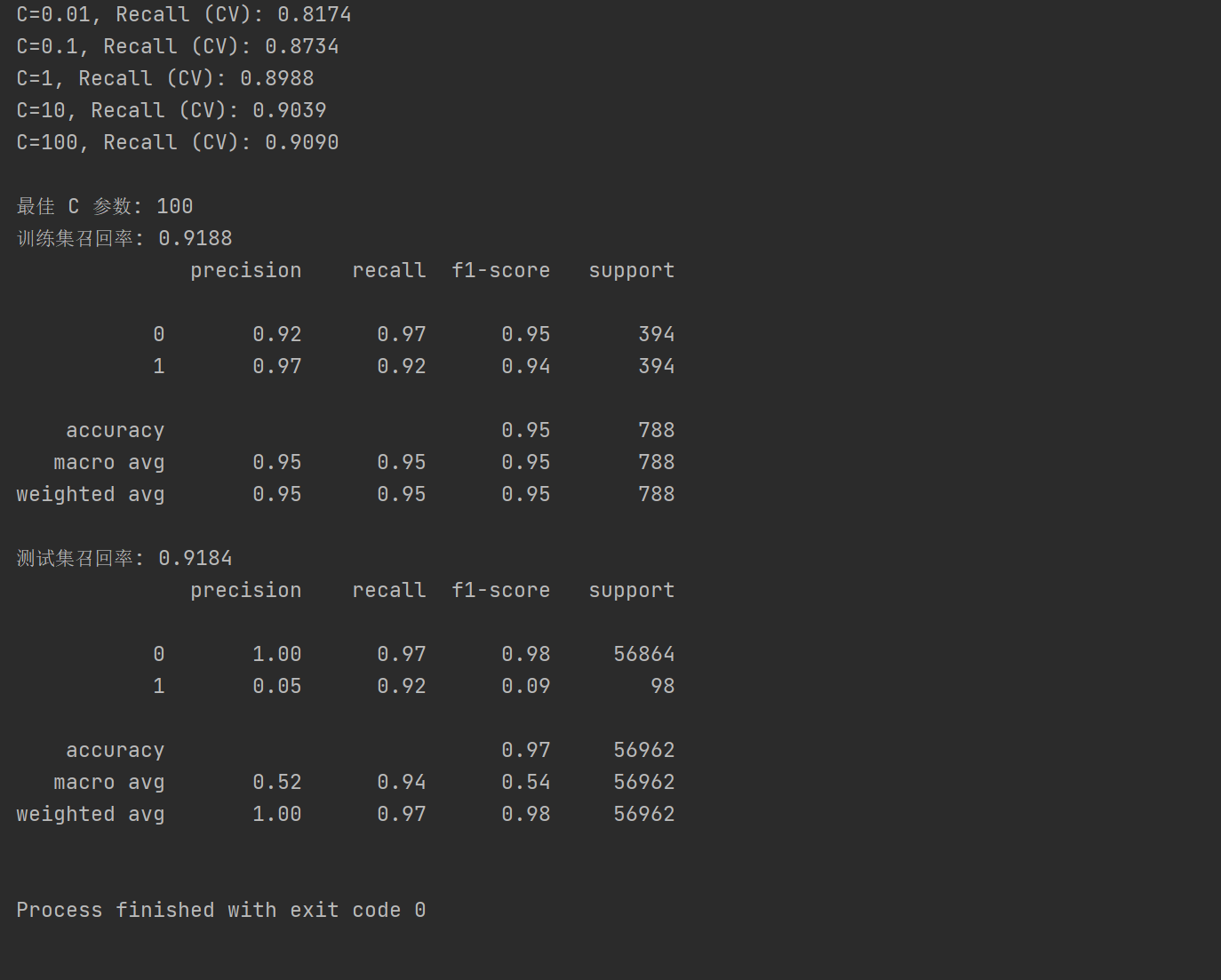
    print(f"C={c}, Recall (CV): {score_mean:.4f}")

# 找到最佳 C
best_c = c_param_range[scores.index(max(scores))]
print(f"\n最佳 C 参数: {best_c}")

# 用最佳 C 训练最终模型
final_pipeline = Pipeline([
    ('scaler', StandardScaler()),
    ('lr', LogisticRegression(C=best_c, penalty='l2', solver='lbfgs', max_iter=1000))
])

# 模型训练
final_pipeline.fit(data_c_x, data_c_y)
# 训练集预测
data_c_pred = final_pipeline.predict(data_c_x)
train_recall = recall_score(data_c_y, data_c_pred)
print(f"训练集召回率: {train_recall:.4f}")
print(classification_report(data_c_y, data_c_pred))
# 测试集预测
y_pred = final_pipeline.predict(X_test)
test_recall = recall_score(y_test, y_pred)
print(f"测试集召回率: {test_recall:.4f}")
print(classification_report(y_test, y_pred))

运行结果：