【论文精读】Instance-Dependent Partial Label Learning

该论文首次提出 ID-PLL 的概念并给出了解决方案 VALEN

Abstract

Partial label learning (PLL) is a typical weakly supervised learning problem, where each training example is associated with a set of candidate labels among which only one is true.

PLL 问题的定义

Most existing PLL approaches assume that the incorrect labels in each training example are randomly picked as the candidate labels. However, this assumption is not realistic since the candidate labels are always instance-dependent.

一般 PLL 问题的局限

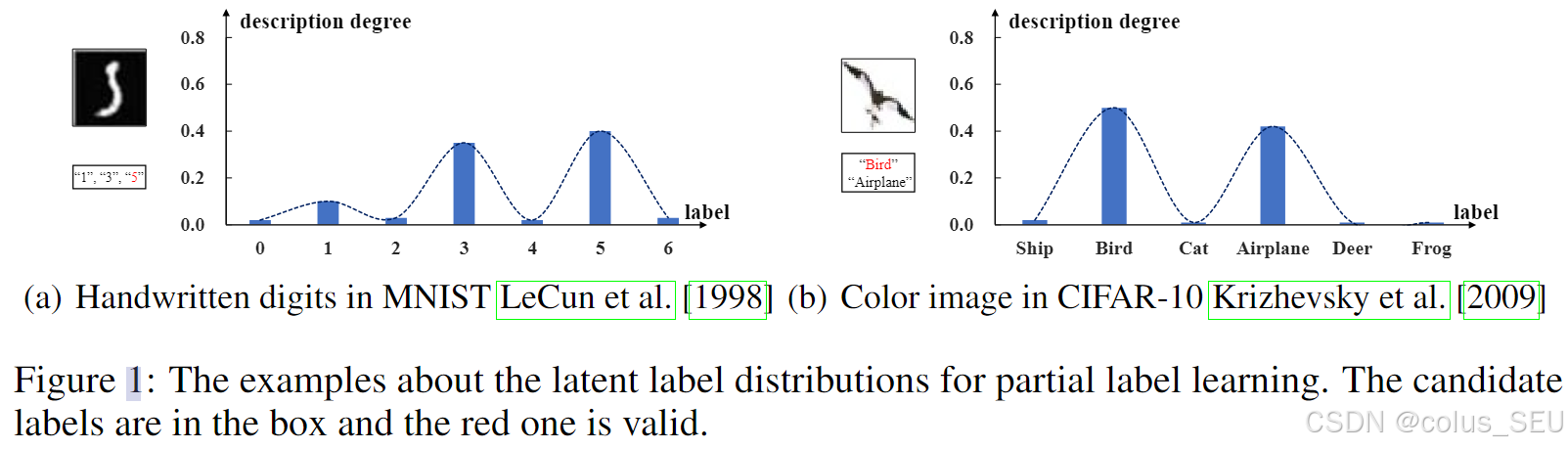
In this paper, we consider instance-dependent PLL and assume that each example is associated with a latent label distribution constituted by the real number of each label, representing the degree to each label describing the feature. The incorrect label with a high degree is more likely to be annotated as the candidate label. Therefore, the latent label distribution is the essential labeling information in partially labeled examples and worth being leveraged for predictive model training.

ID-PLL问题的假设：每个样本都与一个潜在标签分布相关联，该分布由每个标签的实数构成，代表了每个标签描述特征的程度。具有较高程度的错误标签更有可能被标注为候选标签。（说人话就是：每个样本有一个标签置信度分布，该分布未知，且错误标签中置信度高的更可能是候选标签，如figure1中所示。）

Motivated by this consideration, we propose a novel PLL method that recovers the label distribution as a label enhancement (LE) process and trains the predictive model iteratively in every epoch. Specifically, we assume the true posterior density of the latent label distribution takes on the variational approximate Dirichlet density parameterized by an inference model. Then the evidence lower bound is deduced for optimizing the inference model and the label distributions generated from the variational posterior are utilized for training the predictive model.

该论文中的方法将标签分布恢复作为一个标签增强 (LE) 过程，并在每个 epoch 中迭代地训练预测模型。（说人话就是：训练过程中迭代更新置信度分布。）

具体而言，该论文假设潜在标签分布的真实后验密度服从由推理模型参数化的变分近似狄利克雷分布。

然后推导出证据下界（ELBO）用于优化推理模型，并且利用从变分后验生成的标签分布来训练预测模型。

Experiments on benchmark and real-world datasets validate the effectiveness of the proposed method.

（Introduction 省略，其实就是 Abstract 的详细表述）

Method

Problem Formulation

Let \mathcal{X} = \mathbb{R}^q be the q-dimensional instance space and \mathcal{Y} = \{y_1, y_2, \dots, y_c\} be the label space with c class labels.

定义了 Instance 和 Label 空间。

Given the PLL training set \mathcal{D} = \{(\boldsymbol{x}_i, S_i)|1 \leq i \leq n\} where \boldsymbol{x}_i denotes the q-dimensional instance and S_i \subseteq \mathcal{Y} denotes the candidate label set associated with \boldsymbol{x}_i.

定义了训练集。定义了实例 \boldsymbol{x_i} 的候选集。

Note that S_i contains the correct label of \boldsymbol{x}_i and the task of PLL is to induce a multi-class classifier f: \mathcal{X} \mapsto \mathcal{Y} from \mathcal{D}. For each PLL training example (\boldsymbol{x}_i, S_i), we use the logical label vector \boldsymbol{l}_i = [l_i^{y_1}, l_i^{y_2}, \dots, l_i^{y_c}]^\top \in \{0, 1\}^c to represent whether y_j is the candidate label, i.e., l_i^{y_j} = 1 if y_j \in S_i, otherwise l_i^{y_j} = 0.

定义了候选标签向量 \boldsymbol{l_i} 。Multi-class classifier 表示多选一的分类器。

\color{#f8cbad}{\text{The label distribution}} of \boldsymbol{x}_i is denoted by \boldsymbol{d}i = [d_i^{y_1}, d_i^{y_2}, \dots, d_i^{y_c}]^\top \in [0, 1]^c where \sum{j=1}^c d_i^{y_j} = 1.

定义了实例 \boldsymbol{x_i} 的标签置信度分布。

Then \mathbf{L} = [\boldsymbol{l}_1, \boldsymbol{l}_2, \dots, \boldsymbol{l}_n] and \mathbf{D} = [\boldsymbol{d}_1, \boldsymbol{d}_2, \dots, \boldsymbol{d}_n] represent the \color{#f8cbad}{\text{logical label matrix}} and \color{#f8cbad}{\text{label distribution matrix}}, respectively.

定义了候选标签矩阵和标签置信度分布矩阵。

Warm-up Training

The predictive model \boldsymbol{\theta} is trained on partially labeled examples by minimizing the following PLL minimal loss function:

\\color{red} \\mathcal{L}_{min} = \\sum_{i=1}\^{n} \\min_{y_j \\in S_i} \\ell\\left(f(\\boldsymbol{x}_i), \\boldsymbol{e}\^{y_j}\\right), \\tag{1}

where \ell is cross-entropy loss and \boldsymbol{e}^\mathcal{Y} = \{\boldsymbol{e}^{y_j}: y_j \in \mathcal{Y}\} denotes the standard canonical vector in \mathbb{R}^c, i.e., the j-element in \boldsymbol{e}^{y_j} equals 1 and others equal 0. The \min operator in Eq. (1) is replaced by using the current predictions for slightly weighting on the possible labels in warm-up training. Then we could extract the feature \boldsymbol{\phi} of each \boldsymbol{x} via using the predictive model.

该损失函数来自论文 PRODEN：[2002.08053] Progressive Identification of True Labels for Partial-Label Learning

只考虑候选标签中的最小损失，计算举例如下：

假设：类别数 c=3（标签 \mathcal{Y}=\{猫, 狗, 鸟\}，对应索引 1/2/3）。样本 \boldsymbol{x}_i 是一张猫的图片，候选标签集合 S_i=\{猫, 狗\}。模型对该样本的预测输出（softmax后）： f(\boldsymbol{x}_i) = [0.7, 0.2, 0.1] 。则交叉熵损失 \ell(p, \boldsymbol{e}^{y_j}) ，即预测分布 p 与独热标签 \boldsymbol{e}^{y_j} 的差异计算如下：

遍历候选标签 S_i 中的每个标签，计算对应损失：

候选标签「猫」（y_j= 猫，对应 \boldsymbol{e}^{猫} = [1, 0, 0]）： \ell(f(\boldsymbol{x}_i), \boldsymbol{e}^{猫}) = -[1 \cdot \ln 0.7 + 0 \cdot \ln 0.2 + 0 \cdot \ln 0.1] \approx 0.357

候选标签「狗」（y_j= 狗，对应 \boldsymbol{e}^{狗} = [0, 1, 0]）： \ell(f(\boldsymbol{x}_i), \boldsymbol{e}^{狗}) = -[0 \cdot \ln 0.7 + 1 \cdot \ln 0.2 + 0 \cdot \ln 0.1] \approx 1.609

取候选标签中的最小损失： \min\{0.357, 1.609\} = 0.357

对所有样本重复上述步骤，求和得到总损失 \mathcal{L}_{min}，反向传播更新模型。

Warm-up 训练阶段，使用该最小交叉熵损失训练预测模型，大概 10 个 epoch 左右（这是超参，可调）。预测模型初步学习到了样本的特征表示 \boldsymbol{\phi} 以及候选标签的置信度分布，该特征表示用于后续的图构建。

完成 Warm-up 之后，才进入主训练阶段，包括：Label Enhancement + Classifier Training.

Label Enhancement

We assume that the \color{#f8cbad}{\text{prior density}} p(\boldsymbol{d}) is a Dirichlet with \hat{\boldsymbol{\alpha}}, i.e., p(\boldsymbol{d}) = Dir(\boldsymbol{d} \mid \hat{\boldsymbol{\alpha}}) where \hat{\boldsymbol{\alpha}} = [\varepsilon, \varepsilon, \dots, \varepsilon]^\top is a c-dimensional vector with a minor value \varepsilon. Then we let the prior density p(\mathbf{D}) be the product of each Dirichlet

\\color{red} p(\\mathbf{D}) = \\prod_{i=1}\^{n} Dir(\\boldsymbol{d}_i \\mid \\hat{\\boldsymbol{\\alpha}}). \\tag{2}

首先给出先验假设，定义了潜在标签的先验概率密度分布。

当狄利克雷分布的参数 \hat{\alpha} = [\epsilon, \dots, \epsilon] 中的 \epsilon 很小（通常 <1）时，该分布生成的样本（即潜在标签分布 d_i）会倾向于集中在单纯形的顶点。这意味着分布的大部分概率质量会集中在某一个或极少数几个标签上，而其他标签的概率接近 0。这符合论文的假设，即每个样本虽然有多个候选标签，但只有一个是真标签，或者只有少数标签具有较高的置信度。因此，真实的潜在标签分布应该是"尖锐"的，而不是"平坦"的。

p(\mathbf{D}) 代表整个训练集中所有 n 个样本的标签分布矩阵 \mathbf{D} = [\boldsymbol{d}_1, \boldsymbol{d}_2, ..., \boldsymbol{d}n] 的联合概率密度。公式中的连乘符号 \prod{i=1}^{n} 表示模型假设各个样本 x_i 的潜在标签分布 \boldsymbol{d}_i 之间是相互独立的。每个样本的概率 Dir(\boldsymbol{d}_i \mid \hat{\boldsymbol{\alpha}}) 相乘，将复杂的整体分布简化为单个样本分布的乘积。

We consider the topological information of the feature space, which is represented by the \color{#f8cbad}{\text{affinity graph}}（亲和图）G = (V, E, \mathbf{A}). Here, the feature vector \boldsymbol{\phi}_i of each example could be extracted from the predictive model \boldsymbol{\theta} in current epoch, V = \{\boldsymbol{\phi}_i \mid 1 \leq i \leq n\} corresponds to the vertex set consisting of feature vectors, E = \{(\boldsymbol{\phi}i, \boldsymbol{\phi}j) \mid 1 \leq i \neq j \leq n\} corresponds to the edge set, and a sparse adjacency matrix \mathbf{A} = [a{ij}]{n \times n} can be obtained by

a_{ij} = \\begin{cases} 1 \& \\text{if } \\boldsymbol{\\phi}_i \\in \\mathcal{N}(\\boldsymbol{\\phi}_j) \\\\ 0 \& \\text{otherwise} \\end{cases}, \\tag{3}

where \mathcal{N}(\boldsymbol{\phi}_j) is the set for k-nearest neighbors of \boldsymbol{\phi}_j and the diagonal elements of \mathbf{A} are set to 1. Let features matrix \boldsymbol{\Phi} = [\boldsymbol{\phi}_1, \boldsymbol{\phi}_2, \dots, \boldsymbol{\phi}_n], adjacency matrix \mathbf{A} and logical labels \mathbf{L} be \color{#f8cbad}{\text{observed matrix}}, VALEN aims to infer the \color{#f8cbad}{\text{posterior density}} p(\mathbf{D} \mid \mathbf{L}, \boldsymbol{\Phi}, \mathbf{A}). As the computation of the exact posterior density p(\mathbf{D} \mid \mathbf{L}, \boldsymbol{\Phi}, \mathbf{A}) is intractable, a fixed-form density q(\mathbf{D} \mid \mathbf{L}, \boldsymbol{\Phi}, \mathbf{A}) is employed to approximate the true posterior. We let the approximate posterior be the product of each Dirichlet parameterized by a vector \boldsymbol{\alpha}_i = [\alpha_i^1, \alpha_i^2, \dots, \alpha_i^c]^\top:

\\color{red} q_{\\boldsymbol{w}}\\left(\\mathbf{D} \\mid \\mathbf{L}, \\boldsymbol{\\Phi}, \\mathbf{A}\\right) = \\prod_{i=1}\^{n} Dir\\left(\\boldsymbol{d}_i \\mid \\boldsymbol{\\alpha}_i\\right). \\tag{4}

Here, the parameters \boldsymbol{\Delta} = [\boldsymbol{\alpha}_1, \boldsymbol{\alpha}_2, \dots, \boldsymbol{\alpha}_n] are outputs of the inference model parameterized by \boldsymbol{w}, which is defined as a two-layer GCN（图卷积网络） by \color{red} \text{GCN}(\mathbf{L}, \boldsymbol{\Phi}, \mathbf{A}) = \tilde{\mathbf{A}}\text{ReLU}\left(\tilde{\mathbf{A}}\mathbf{Z}\mathbf{W}_0\right)\mathbf{W}_1, with \mathbf{Z} = [\boldsymbol{\Phi}; \mathbf{L}] and weight \mathbf{W}_0, \mathbf{W}_1. Here \tilde{\mathbf{A}} = \hat{\mathbf{A}}^{-\frac{1}{2}}\mathbf{A}\hat{\mathbf{A}}^{-\frac{1}{2}} is the symmetrically normalized weight matrix where \hat{\mathbf{A}} is the degree matrix of \mathbf{A}.

然后定义了变分近似后验。

先利用 Warm-up training 阶段得到的特征向量构建亲和图 G = (V, E, \mathbf{A})。其中 V 是特征向量对应的点，E 是边，\mathbf{A} 是稀疏邻接矩阵，由 k 近邻定义。

用特征矩阵 \boldsymbol{\Phi} = [\boldsymbol{\phi}_1, \boldsymbol{\phi}_2, \dots, \boldsymbol{\phi}_n]，邻接矩阵 \mathbf{A}，候选标签矩阵 \mathbf{L} 作为参数，VALEN 希望推出标签分布矩阵的后验概率密度：p(\mathbf{D} \mid \mathbf{L}, \boldsymbol{\Phi}, \mathbf{A})。

但是该后验概率无法准确计算出来，因此使用 q_{\boldsymbol{w}}(\mathbf{D} \mid \mathbf{L}, \boldsymbol{\Phi}, \mathbf{A}) 来估计它，其定义如公式4。这里的 \boldsymbol{w} 表示的是一个由两层 GCN 构成的推理模型的参数。

公式4中先使用两层 GCN 得到狄利克雷分布的参数 \boldsymbol{\Delta} ，然后代入狄利克雷分布的概率密度函数即可求解。

两层 GCN 的计算逻辑是：\mathbf{Z} = [\boldsymbol{\Phi}; \mathbf{L}] 把 视觉特征 \boldsymbol{\Phi} 和 候选标签 \mathbf{L} 拼在了一起作为输入，包含了特征和候选标签，这是每个节点的"身份证"。矩阵 \mathbf{W}_0, \mathbf{W}_1 是可学习的参数，作用是对特征进行提炼和维度变换。矩阵 \tilde{\mathbf{A}} (Normalized Adjacency Matrix) 包含了图的结构信息（谁连着谁），\tilde{\mathbf{A}} \times \mathbf{Z} 的物理意义："我的特征 = 我邻居特征的加权平均"。公式里的 \hat{\mathbf{A}}^{-\frac{1}{2}} 是为了归一化（Normalized）来保持数学上的数值稳定性，通俗解释就是如果一个节点是"交际花"，连了 1000 个邻居，如果不做归一化，它的特征值加起来会爆炸大；如果一个节点只有一个邻居，数值就很小。归一化就是让"大家说话的分量平均一点"，不要因为朋友多就嗓门特别大。

这里用 GCN 的原因是基于该假设：相似的样本，即特征相似，应该有相似的标签。

By following the Variational Bayes techniques, a lower bound on the marginal likelihood of the model is derived which ensures that q_{\boldsymbol{w}}(\mathbf{D} \mid \mathbf{L}, \boldsymbol{\Phi}, \mathbf{A}) is as close as possible to p(\mathbf{D} \mid \mathbf{L}, \boldsymbol{\Phi}, \mathbf{A}). For logical label matrix \mathbf{L}, feature matrix \boldsymbol{\Phi}, and the corresponding \mathbf{A}, the log marginal probability can be decomposed as follows:

\\color{red} \\log p(\\mathbf{L}, \\boldsymbol{\\Phi}, \\mathbf{A}) = \\mathcal{L}_{ELBO} + \\mathrm{KL}\\!\\left\[q_{\\boldsymbol{w}}(\\mathbf{D} \\mid \\mathbf{L}, \\boldsymbol{\\Phi}, \\mathbf{A}) \\parallel p(\\mathbf{D} \\mid \\mathbf{L}, \\boldsymbol{\\Phi}, \\mathbf{A})\\right\]. \\tag{5}

where

\\color{red} \\mathcal{L}_{ELBO} = \\mathbb{E}_{q_{\\boldsymbol{w}}(\\mathbf{D} \\mid \\mathbf{L}, \\boldsymbol{\\Phi}, \\mathbf{A})}\\big\[\\log p(\\mathbf{L}, \\boldsymbol{\\Phi}, \\mathbf{A} \\mid \\mathbf{D})\\big\] - \\mathrm{KL}\\!\\left\[q_{\\boldsymbol{w}}(\\mathbf{D} \\mid \\mathbf{L}, \\boldsymbol{\\Phi}, \\mathbf{A}) \\parallel p(\\mathbf{D})\\right\]. \\tag{6}

Due to the non-negative property of KL divergence, the first term \mathcal{L}{ELBO} constitutes a lower bound of \log p(\mathbf{L}, \boldsymbol{\Phi}, \mathbf{A}), which is often called as evidence lower bound (ELBO), i.e., \log p(\mathbf{L}, \boldsymbol{\Phi}, \mathbf{A}) \geq \mathcal{L}{ELBO}.

还是之前提到的，我们的目标是求出标签分布矩阵的真实后验 p(\mathbf{D} \mid \mathbf{L}, \boldsymbol{\Phi}, \mathbf{A})，即"看了这张图和候选标签后，它的真实标签分布应该是啥？"。但是，直接用贝叶斯公式计算这个后验概率是不可能的（Intractable） ，因为分母（边缘概率 p(\mathbf{L}, \boldsymbol{\Phi}, \mathbf{A})）需要对所有可能的 \mathbf{D} 进行积分，在高维空间中无法计算。因此，该论文采用变分推断 的方法：既然求不出真实的 p，那我们就找一个简单的分布 q_{\boldsymbol{w}}（即 GCN 输出的那个分布），让它尽可能逼近真实的 p 。即找出其界限。

首先对对数边缘概率进行计算，推导如下：

基于概率的基本乘法公式可以得到：
$\\log p(\\mathbf{L}, \\boldsymbol{\\Phi}, \\mathbf{A}) = \\log p(\\mathbf{D}, \\mathbf{L}, \\boldsymbol{\\Phi}, \\mathbf{A}) - \\log p(\\mathbf{D} \\mid \\mathbf{L}, \\boldsymbol{\\Phi}, \\mathbf{A})$
为了引入变分分布 q_w(D|L,\Phi,A)，等式两边同时乘以该分布，并对 D 进行积分（对于连续变量）：
$\\int_{\\mathbf{D}} q_w(\\mathbf{D} \\mid \\mathbf{L}, \\boldsymbol{\\Phi}, \\mathbf{A}) \\log p(\\mathbf{L}, \\boldsymbol{\\Phi}, \\mathbf{A}) d\\mathbf{D} = \\int_{\\mathbf{D}} q_w(\\mathbf{D} \\mid \\mathbf{L}, \\boldsymbol{\\Phi}, \\mathbf{A}) \\big( \\log p(\\mathbf{D}, \\mathbf{L}, \\boldsymbol{\\Phi}, \\mathbf{A}) - \\log p(\\mathbf{D} \\mid \\mathbf{L}, \\boldsymbol{\\Phi}, \\mathbf{A}) \\big) d\\mathbf{D}.$
对于左边：由于 \log p(\mathbf{L}, \boldsymbol{\Phi}, \mathbf{A}) 不依赖于变量 \mathbf{D}，它相对于积分来说是常数。且概率密度函数的积分为 1（\int q_w d\mathbf{D} = 1）；

对于右边：引入 KL 散度公式：\mathrm{KL}(P \parallel Q) = \int_{-\infty}^{+\infty} p(x) \log \frac{p(x)}{q(x)} \mathrm{d}x ；

因此有：
$\\begin{aligned} \\log p(\\mathbf{L}, \\boldsymbol{\\Phi}, \\mathbf{A}) \&= \\int_{\\mathbf{D}} q_w(\\mathbf{D} \\mid \\mathbf{L}, \\boldsymbol{\\Phi}, \\mathbf{A}) \\big( \\log p(\\mathbf{D}, \\mathbf{L}, \\boldsymbol{\\Phi}, \\mathbf{A}) - \\log p(\\mathbf{D} \\mid \\mathbf{L}, \\boldsymbol{\\Phi}, \\mathbf{A}) \\big) d\\mathbf{D} \\\\ \&= \\int_{\\mathbf{D}} q_w(\\mathbf{D} \\mid \\mathbf{L}, \\boldsymbol{\\Phi}, \\mathbf{A}) \\big( \\log \\frac{p(\\mathbf{D}, \\mathbf{L}, \\boldsymbol{\\Phi}, \\mathbf{A})}{q_w(\\mathbf{D} \\mid \\mathbf{L}, \\boldsymbol{\\Phi}, \\mathbf{A})} - \\log \\frac{p(\\mathbf{D} \\mid \\mathbf{L}, \\boldsymbol{\\Phi}, \\mathbf{A})}{q_w(\\mathbf{D} \\mid \\mathbf{L}, \\boldsymbol{\\Phi}, \\mathbf{A})} \\big) d\\mathbf{D} \\\\ \&= \\int_{\\mathbf{D}} q_w(\\mathbf{D} \\mid \\mathbf{L}, \\boldsymbol{\\Phi}, \\mathbf{A}) \\log \\frac{p(\\mathbf{D}, \\mathbf{L}, \\boldsymbol{\\Phi}, \\mathbf{A})}{q_w(\\mathbf{D} \\mid \\mathbf{L}, \\boldsymbol{\\Phi}, \\mathbf{A})} d\\mathbf{D} + \\mathrm{KL}\\big\[ q_w(\\mathbf{D} \\mid \\mathbf{L}, \\boldsymbol{\\Phi}, \\mathbf{A}) \\parallel p(\\mathbf{D} \\mid \\mathbf{L}, \\boldsymbol{\\Phi}, \\mathbf{A}) \\big\]. \\end{aligned}$
该公式中，右边第一项为 ELBO（变分下界/证据下界）
$\\begin{aligned} \\mathcal{L}_{ELBO} \&= \\int_{\\mathbf{D}} q_w(\\mathbf{D} \\mid \\mathbf{L}, \\boldsymbol{\\Phi}, \\mathbf{A}) \\log \\frac{p(\\mathbf{D}, \\mathbf{L}, \\boldsymbol{\\Phi}, \\mathbf{A})}{q_w(\\mathbf{D} \\mid \\mathbf{L}, \\boldsymbol{\\Phi}, \\mathbf{A})} d\\mathbf{D} \\\\ \&= \\int_{\\mathbf{D}} q_w(\\mathbf{D} \\mid \\mathbf{L}, \\boldsymbol{\\Phi}, \\mathbf{A}) \\big( \\log \\frac{p(\\mathbf{D}) p(\\mathbf{L}, \\boldsymbol{\\Phi}, \\mathbf{A} \\mid \\mathbf{D})}{q_w(\\mathbf{D} \\mid \\mathbf{L}, \\boldsymbol{\\Phi}, \\mathbf{A})} \\big) d\\mathbf{D} \\\\ \&= \\mathbb{E}_{q_w(\\mathbf{D} \\mid \\mathbf{L}, \\boldsymbol{\\Phi}, \\mathbf{A})} \\big\[ \\log p(\\mathbf{L}, \\boldsymbol{\\Phi}, \\mathbf{A} \\mid \\mathbf{D}) \\big\] - \\mathrm{KL}\\big\[ q_w(\\mathbf{D} \\mid \\mathbf{L}, \\boldsymbol{\\Phi}, \\mathbf{A}) \\parallel p(\\mathbf{D}) \\big\]. \\end{aligned}$
最终得到： \log p(\mathbf{L}, \boldsymbol{\Phi}, \mathbf{A}) = \mathcal{L}_{ELBO} + \mathrm{KL}\big[ q_w(\mathbf{D} \mid \mathbf{L}, \boldsymbol{\Phi}, \mathbf{A}) \parallel p(\mathbf{D} \mid \mathbf{L}, \boldsymbol{\Phi}, \mathbf{A}) \big]. \tag{5}

由于 KL 散度是非负的，从公式5我们可知：

左边是固定的：观测数据的对数概率（Log Likelihood）是一个常数。

右边是此消彼长的 ：既然总和固定，如果我们能最大化 \mathcal{L}_{ELBO} ，那么 \mathrm{KL}[q \parallel p]（即近似分布 q 与真实分布 p 的差距）就会被迫最小化。

结论：只要拼命优化 \mathcal{L}_{ELBO}，我们就能让 GCN 学到的分布无限接近真实的标签分布。

According to Eq. (2) and Eq. (4), the KL divergence in Eq. (6) can be analytically calculated as follows:

\\begin{aligned} \\mathrm{KL}\\left(q_{\\boldsymbol{w}}(\\mathbf{D} \\mid \\mathbf{L}, \\boldsymbol{\\Phi}, \\mathbf{A}) \\parallel p(\\mathbf{D})\\right) \&= \\sum_{i=1}\^{n} \\Bigg( \\log \\Gamma\\left(\\sum_{j=1}\^{c} \\alpha_i\^j\\right) - \\sum_{j=1}\^{c} \\log \\Gamma\\left(\\alpha_i\^j\\right) \\\\ \&\\quad - \\log \\Gamma(c \\cdot \\varepsilon) + c \\log \\Gamma(\\varepsilon) + \\sum_{j=1}\^{c} \\left(\\alpha_i\^j - \\varepsilon\\right) \\left( \\psi\\left(\\alpha_i\^j\\right) - \\psi\\left(\\sum_{j=1}\^{c} \\alpha_i\^j\\right) \\right) \\Bigg), \\end{aligned} \\tag{7}

where \Gamma(\cdot) and \psi(\cdot) are Gamma function and Digamma function, respectively.

As the first part of Eq. (6) is intractable, we employ the implicit reparameterization trick [Figurnov et al. 2018] to approximate it by Monte Carlo (MC) estimation. Inspired by [Kipf and Welling 2016], we simply drop the dependence on \boldsymbol{\Phi}:

\\begin{aligned} p(\\mathbf{L} \\mid \\mathbf{A}, \\mathbf{D}) \&= \\prod_{i=1}\^{n} p\\left(\\boldsymbol{l}_i \\mid \\mathbf{A}, \\mathbf{D}\\right), \\\\ p(\\mathbf{A} \\mid \\mathbf{D}) \&= \\prod_{i=1}\^{n} \\prod_{j=1}\^{n} p\\left(a_{ij} \\mid \\boldsymbol{d}_i, \\boldsymbol{d}_j\\right), \\text{ with } p\\left(a_{ij} = 1 \\mid \\boldsymbol{d}_i, \\boldsymbol{d}_j\\right) = s\\left(\\boldsymbol{d}_i\^\\top \\boldsymbol{d}_j\\right). \\end{aligned} \\tag{8}

Here, s(\cdot) is the logistic sigmoid function. We further assume that p\left(\boldsymbol{l}_i \mid \mathbf{A}, \mathbf{D}\right) is a multivariate Bernoulli with probabilities \boldsymbol{\tau}_i. In order to simplify the observation model, \mathbf{T}^{(m)} = [\boldsymbol{\tau}_1^{(m)}, \boldsymbol{\tau}_2^{(m)}, \dots, \boldsymbol{\tau}_n^{(m)}] is computed from m-th sampling \mathbf{D}^{(m)} with a three-layer MLP parameterized by \boldsymbol{\eta}. Then the first part of Eq. (6) can be tractable:

\\color{blue} \\begin{aligned} \\mathbb{E}_{q_{\\boldsymbol{w}}(\\mathbf{D} \\mid \\mathbf{L}, \\boldsymbol{\\Phi}, \\mathbf{A})}\\big\[\\log p_{\\boldsymbol{\\eta}}(\\mathbf{L}, \\boldsymbol{\\Phi}, \\mathbf{A} \\mid \\mathbf{D})\\big\] \&= \\frac{1}{M} \\sum_{m=1}\^{M} \\Bigg( \\mathrm{tr}\\left( \\left(\\mathbf{I} - \\mathbf{L}\\right)\^\\top \\log\\left(\\mathbf{I} - \\mathbf{T}\^{(m)}\\right) \\right) \\\\ \&\\quad + \\mathrm{tr}\\left( \\mathbf{L}\^\\top \\log \\mathbf{T}\^{(m)} \\right) - \\left\\lVert \\mathbf{A} - S\\left(\\mathbf{D}\^{(m)} \\mathbf{D}\^{(m)\\top}\\right) \\right\\rVert_F\^2 \\Bigg). \\end{aligned} \\tag{9}

Note that we can use only one MC sample in Eq. (9) during the training process as suggested in [Kingma and Welling 2014], [Xu et al. 2020].

由之前的分析，接下来的任务就是最大化 \mathcal{L}_{ELBO}.
$\\mathcal{L}_{ELBO} = \\underbrace{\\mathbb{E}_{q_{\\boldsymbol{w}}(\\mathbf{D} \\mid \\mathbf{L}, \\boldsymbol{\\Phi}, \\mathbf{A})}\\big\[\\log p(\\mathbf{L}, \\boldsymbol{\\Phi}, \\mathbf{A} \\mid \\mathbf{D})\\big\]}_{\\text{第一项：重构能力}} - \\underbrace{\\mathrm{KL}\\!\\left\[q_{\\boldsymbol{w}}(\\mathbf{D} \\mid \\mathbf{L}, \\boldsymbol{\\Phi}, \\mathbf{A}) \\parallel p(\\mathbf{D})\\right\]}_{\\text{第二项：先验约束}}.$
KL 散度项表示的是先验约束：

直觉：这是在计算------"你生成的分布 \mathbf{D} 和我预设的先验规则（稀疏分布）差别有多大？"

作用：它迫使生成的 \mathbf{D} 保持稀疏性。我们在先验中设置了 \epsilon 很小，假设真实分布是尖锐的（one-hot 附近）。这一项会惩罚那些"模棱两可"（比如均匀分布）的预测，防止模型过拟合数据中的噪声。

计算：代入公式2和4的定义以及狄利克雷概率密度函数的定义即可推导，结果为公式7，具体推导如下：

公式 (7) 计算的是两个狄利克雷分布之间的 KL 散度。假设我们有两个狄利克雷分布：

近似后验分布 (Posterior) q(\boldsymbol{d})：参数为 \boldsymbol{\alpha} = [\alpha_1, \dots, \alpha_c]。

先验分布 (Prior) p(\boldsymbol{d})：参数为 \hat{\boldsymbol{\alpha}} = [\epsilon, \dots, \epsilon] （即论文中的 \beta_j = \epsilon）。

狄利克雷分布的概率密度函数 (PDF) 为：Dir(\boldsymbol{d}|\boldsymbol{\alpha}) = \frac{1}{B(\boldsymbol{\alpha})} \prod_{j=1}^{c} (d^j)^{\alpha_j - 1}

其中 B(\boldsymbol{\alpha}) 是多变量贝塔函数：B(\boldsymbol{\alpha}) = \frac{\prod_{j=1}^{c} \Gamma(\alpha_j)}{\Gamma(\sum_{j=1}^{c} \alpha_j)} = \frac{\prod \Gamma(\alpha_j)}{\Gamma(S_\alpha)}, \quad \text{令 } S_\alpha = \sum_{j=1}^c \alpha_j

KL 散度积分形式的定义是：KL(q \| p) = \int q(\boldsymbol{d}) \log \frac{q(\boldsymbol{d})}{p(\boldsymbol{d})} d\boldsymbol{d} = \mathbb{E}_{q} [\log q(\boldsymbol{d}) - \log p(\boldsymbol{d})]

我们先分别写出 \log q(\boldsymbol{d}) 和 \log p(\boldsymbol{d})：

对于 q(\boldsymbol{d})：\log q(\boldsymbol{d}) = \log \left( \frac{1}{B(\boldsymbol{\alpha})} \prod_{j=1}^{c} (d^j)^{\alpha_j - 1} \right) = -\log B(\boldsymbol{\alpha}) + \sum_{j=1}^{c} (\alpha_j - 1) \log d^j

对于 p(\boldsymbol{d})：\log p(\boldsymbol{d}) = -\log B(\hat{\boldsymbol{\alpha}}) + \sum_{j=1}^{c} (\hat{\alpha}_j - 1) \log d^j

将上述两式相减并求期望：
$\\begin{aligned} \\mathrm{KL}(q \\\| p) \&= \\mathbb{E}_{q} \\left\[ -\\log B(\\boldsymbol{\\alpha}) + \\sum (\\alpha_j - 1) \\log d\^j - \\left( -\\log B(\\hat{\\boldsymbol{\\alpha}}) + \\sum (\\hat{\\alpha}_j - 1) \\log d\^j \\right) \\right\] \\\\ \&= \\underbrace{-\\log B(\\boldsymbol{\\alpha}) + \\log B(\\hat{\\boldsymbol{\\alpha}})}_{\\text{常数项}} + \\sum_{j=1}\^{c} (\\alpha_j - \\hat{\\alpha}_j) \\underbrace{\\mathbb{E}_{q}\[\\log d\^j\]}_{\\text{关键期望}} \\end{aligned}$
**关键数学性质：**对于服从 Dir(\boldsymbol{\alpha}) 的变量 \boldsymbol{d}，\log d^j 的期望由 Digamma 函数 \psi(\cdot) 给出：
$\\mathbb{E}_{q}\[\\log d\^j\] = \\psi(\\alpha_j) - \\psi\\left(\\sum_{k=1}\^{c} \\alpha_k\\right) = \\psi(\\alpha_j) - \\psi(S_\\alpha)$
将期望公式代回 KL 散度表达式，并代入论文的具体设置：

后验参数 \boldsymbol{\alpha} 对应论文中的 \alpha_i^j。

先验参数 \hat{\boldsymbol{\alpha}} 对应论文中的 \epsilon（所有分量均为 \epsilon）。

因此，\sum \hat{\alpha}j = \sum{j=1}^c \epsilon = c \cdot \epsilon。

步骤 1：展开 Beta 函数项
$\\begin{aligned} -\\log B(\\boldsymbol{\\alpha}) \&= -\\log \\frac{\\prod \\Gamma(\\alpha_j)}{\\Gamma(\\sum \\alpha_j)} = \\log \\Gamma\\left(\\sum \\alpha_j\\right) - \\sum \\log \\Gamma(\\alpha_j) \\\\ \\log B(\\hat{\\boldsymbol{\\alpha}}) \&= \\log \\frac{\\prod \\Gamma(\\epsilon)}{\\Gamma(\\sum \\epsilon)} = \\log \\frac{(\\Gamma(\\epsilon))\^c}{\\Gamma(c\\epsilon)} = c \\log \\Gamma(\\epsilon) - \\log \\Gamma(c\\epsilon) \\end{aligned}$
这对应了公式 (7) 中的前四项。

步骤 2：展开期望项
$\\sum_{j=1}\^{c} (\\alpha_j - \\hat{\\alpha}_j) \\mathbb{E}\[\\log d\^j\] = \\sum_{j=1}\^{c} (\\alpha_j - \\epsilon) \\left( \\psi(\\alpha_j) - \\psi\\left(\\sum_{k=1}\^{c} \\alpha_k\\right) \\right)$
这对应了公式 (7) 中的最后一项。

将 1 和 2 的结果相加，并对所有 n 个样本求和（因为样本间独立），即可得到论文中的公式7：
$\\color{blue} \\begin{aligned} \\mathrm{KL}(q \\\| p) = \\sum_{i=1}\^{n} \\Bigg( \& \\underbrace{\\log \\Gamma\\left(\\sum_{j=1}\^{c} \\alpha_i\^j\\right) - \\sum_{j=1}\^{c} \\log \\Gamma(\\alpha_i\^j)}_{\\text{来自 } -\\log B(\\boldsymbol{\\alpha}_i)} \\underbrace{- \\log \\Gamma(c \\cdot \\epsilon) + c \\log \\Gamma(\\epsilon)}_{\\text{来自 } \\log B(\\hat{\\boldsymbol{\\alpha}})} + \\underbrace{\\sum_{j=1}\^{c} (\\alpha_i\^j - \\epsilon) \\left( \\psi(\\alpha_i\^j) - \\psi\\left(\\sum_{k=1}\^{c} \\alpha_i\^k\\right) \\right)}_{\\text{来自期望项}} \\Bigg) \\end{aligned}$

期望项表示的是重构标签分布的能力：

直觉：这是在问模型------"如果你猜的标签分布 \mathbf{D} 是真的，那么看到当前这些数据（标签和图）的概率大不大？"

作用：它迫使生成的 \mathbf{D} 必须忠实于观测数据。例如，如果样本 i 的候选标签里没有"猫"，那么生成的分布 \mathbf{D} 在"猫"这一项上的概率就不能高，否则这一项得分会很低。

但是该项不容易计算。

计算该"重构误差"的核心思想是利用**变分自编码器（VAE）**的解码器（Decoder）逻辑，从生成的潜在标签分布 \mathbf{D} 中"还原"出观测数据（逻辑标签 \mathbf{L} 和图结构 \mathbf{A}）。为了解决积分难算的问题，作者使用了蒙特卡洛采样（MC Estimation）和重参数化技巧（Reparameterization Trick）。

1. 简化与独立性假设 (Eq. 8)

首先，作者需要定义 p(\mathbf{L}, \boldsymbol{\Phi}, \mathbf{A} \mid \mathbf{D})，即给定潜在分布 \mathbf{D} 时，观测数据出现的概率。

忽略特征 \boldsymbol{\Phi}：为了简化计算，作者参考了 Kipf & Welling (2016) 的做法，忽略了对特征 \boldsymbol{\Phi} 的生成依赖，只关注标签 \mathbf{L} 和图结构 \mathbf{A} 的重构。

条件独立性：作者假设 \mathbf{L} 和 \mathbf{A} 的生成过程是相对独立的。

生成标签 \mathbf{L}：\color{blue}p(\mathbf{L} \mid \mathbf{A}, \mathbf{D}) = \prod_{i=1}^{n} p\left(\boldsymbol{l}_i \mid \mathbf{A}, \mathbf{D}\right)。即每个样本的逻辑标签是独立生成的。

生成图结构 \mathbf{A}：p(\mathbf{A} \mid \mathbf{D}) = \prod \prod p(a_{ij} \mid \boldsymbol{d}i, \boldsymbol{d}j)。即图中的边是否存在，取决于两个节点的潜在分布 \boldsymbol{d}i 和 \boldsymbol{d}j 的关系。这里使用了内积解码器（Inner Product Decoder）的思想：如果两个样本的标签分布相似（内积大），它们之间存在边（a{ij}=1）的概率就大。概率由 Sigmoid 函数 s(\cdot) 给出：\color{blue} p(\mathbf{A} \mid \mathbf{D}) = \prod{i=1}^{n} \prod{j=1}^{n} p\left(a{ij} \mid \boldsymbol{d}_i, \boldsymbol{d}j\right), \text{ with } p\left(a{ij} = 1 \mid \boldsymbol{d}_i, \boldsymbol{d}_j\right) = s\left(\boldsymbol{d}_i^\top \boldsymbol{d}_j\right).

由以上两个假设，得到：
$p(\\mathbf{L}, \\boldsymbol{\\Phi}, \\mathbf{A} \\mid \\mathbf{D}) = \\log p(\\mathbf{L}, \\mathbf{A} \\mid \\mathbf{D}) = \\underbrace{\\log p(\\mathbf{L} \\mid \\mathbf{D})}_{\\text{标签重构}} + \\underbrace{\\log p(\\mathbf{A} \\mid \\mathbf{D})}_{\\text{图重构}}$
2. 具体的观测模型 (Observation Model)

为了把上述概率写成具体的数学公式，作者做了以下假设：

逻辑标签 \mathbf{L} 服从多元伯努利分布：因为 \mathbf{L} 中的元素是 0 或 1，这很自然。为了得到伯努利分布的参数（概率值 \boldsymbol{\tau}），作者使用了一个由 \boldsymbol{\eta} 参数化的 三层 MLP（多层感知机）。输入是采样的分布 \mathbf{D}，输出是预测的概率矩阵 \mathbf{T} 。

对于第 i 个样本的第 j 个类别，观测值是 l_{ij} \in \{0, 1\}，预测概率是 \tau_{ij}^{(m)}（即矩阵 \mathbf{T}^{(m)} 的元素）。单个元素的伯努利对数似然为：
$\\log p(l_{ij} \\mid \\tau_{ij}) = l_{ij} \\log \\tau_{ij} + (1 - l_{ij}) \\log (1 - \\tau_{ij})$
对所有样本 i 和类别 j 求和，得到整体的对数似然：
$\\log p(\\mathbf{L} \\mid \\mathbf{D}) = \\sum_{i=1}\^{n} \\sum_{j=1}\^{c} \\left\[ l_{ij} \\log \\tau_{ij} + (1 - l_{ij}) \\log (1 - \\tau_{ij}) \\right\]$

图结构 \mathbf{A} 由点积决定：如前所述，通过 S(\mathbf{D}\mathbf{D}^\top) 计算边的概率。

3. 最终的可计算损失函数 (Eq. 9)

公式 (9) 是将上述概率模型带入对数似然 \log p(\dots) 后推导出的最终计算公式。它利用蒙特卡洛采样（MC Sampling），将不可算的期望 \mathbb{E} 转化为样本的平均值。公式由三部分组成，分别对应两个重构任务：

A. 标签重构部分 (Label Reconstruction)：这一部分是二元交叉熵损失（Binary Cross Entropy, BCE）的矩阵迹形式。

项 1：\sum_{i,j} l_{ij} \log \tau_{ij} = \mathrm{tr}(\mathbf{L}^\top \log \mathbf{T}^{(m)})：对应公式 \sum y \log \hat{y} 中的正类部分。即：若实际上是候选标签 (L=1)，则希望预测概率 T 越大越好。

项 2：\sum_{i,j} (1 - l_{ij}) \log (1 - \tau_{ij}) = \mathrm{tr}((\mathbf{1} - \mathbf{L})^\top \log (\mathbf{1} - \mathbf{T}^{(m)}))：对应公式 \sum (1-y) \log (1-\hat{y}) 中的负类部分。即：若不是候选标签 (L=0)，则希望预测概率 T 越小越好。（对于两个同维矩阵 \mathbf{X} 和 \mathbf{Y}，其对应元素乘积之和（Frobenius 内积）等于 \mathrm{tr}(\mathbf{X}^\top \mathbf{Y})。）

这两个迹运算加起来，本质上就是在计算生成的逻辑标签 \mathbf{T} 与真实观测的逻辑标签 \mathbf{L} 之间的相似度。

B. 图重构部分 (Graph Reconstruction)

项 3：- || \mathbf{A} - S(\mathbf{D}^{(m)} \mathbf{D}^{(m)\top}) ||_F^2

这是一个 F范数（均方误差，MSE）项，使用了均方误差（MSE）作为图重构的损失函数。

它衡量的是真实的邻接矩阵 \mathbf{A} 与根据潜在分布计算出的相似度矩阵 S(\mathbf{D}\mathbf{D}^\top) 之间的距离。

负号表示我们要最大化对数似然，等同于最小化这个重构误差。

这一推导过程将一个复杂的概率生成问题转化为了神经网络可以训练的损失函数：

随机采样一个 \mathbf{D}。

用 MLP 预测标签，算出交叉熵损失（前两项）。

用点积预测图结构，算出均方误差损失（第三项）。

利用蒙特卡洛采样，将它们加起来取平均，就得到了 ELBO 的第一部分。

In addition, VALEN improves the label enhancement by employing the compatibility loss, which enforces that the recovered label distributions should not be completely different from the confidence \zeta(\boldsymbol{x}_i) [Feng et al. 2020], [Lv et al. 2020] estimated by current prediction f(\boldsymbol{x}_i; \boldsymbol{\theta}):

\\color{red} \\mathcal{L}_o = -\\frac{1}{n} \\sum_{i=1}\^{n} \\sum_{j=1}\^{c} \\zeta_j(\\boldsymbol{x}_i) \\log d_i\^{y_j}. \\tag{10}

where

\\zeta_j(\\boldsymbol{x}_i) = \\begin{cases} f_j\\left(\\boldsymbol{x}_i; \\boldsymbol{\\theta}\\right) \\big/ \\sum_{y_k \\in S_i} f_k\\left(\\boldsymbol{x}_i; \\boldsymbol{\\theta}\\right) \& \\text{if } y_j \\in S_i \\\\ 0 \& \\text{otherwise} \\end{cases}. \\tag{11}

Now we can easily get the objective of label enhancement \mathcal{L}_{LE} as follows:

\\color{red} \\mathcal{L}_{LE} = \\lambda \\mathcal{L}_o - \\mathcal{L}_{ELBO}, \\tag{12}

where \lambda is a hyper-parameter. The label distribution matrix \mathbf{D} is sampled from q(\mathbf{D} \mid \mathbf{L}, \boldsymbol{\Phi}, \mathbf{A}), i.e., \boldsymbol{d}_i \sim Dir(\boldsymbol{\alpha}_i). Note that the implicit reparameterization gradient [Figurnov et al. 2018] is employed, which avoids the inversion of the standardization function, which makes the gradients can be computed analytically in backward pass.

除了优化 \mathcal{L}_{ELBO} ，VALEN 算法还通过引入**"兼容性损失"（Compatibility Loss）**来改进标签增强过程。兼容性损失的引入理由在于：虽然 GCN 通过图结构推断出了标签分布 \mathbf{D}，但作者认为这个分布不能完全"凭空想象"，它应该参考当前分类器（Predictive Model f(\cdot; \boldsymbol{\theta})）的意见。

作者首先定义当前分类器对样本 \boldsymbol{x}_i 的"置信度" \zeta(\boldsymbol{x}_i) 为公式 11。这实际上是对分类器输出的一个重新归一化，非候选标签置信度直接设为 0，候选标签置信度的和为 1。兼容性损失函数定义为一个标准的交叉熵损失（Cross-Entropy Loss），见公式10。它把分类器的置信度 \zeta 当作软标签（Soft Target），去指导 GCN 生成的标签分布 \mathbf{D}，确保 GCN 恢复出来的分布 \mathbf{D} 不要偏离分类器的判断太远。这形成了一个闭环反馈：分类器越准，\zeta 越准，进而指导 \mathbf{D} 越准；反之，更准的 \mathbf{D} 又在下一节用于训练分类器。

公式 (12) 给出了标签增强模块最终的损失函数。这里存在一种有趣的权衡（Trade-off）：

-\mathcal{L}_{ELBO}（最大化 ELBO）：这一项由图结构和变分推断驱动。它希望 \mathbf{D} 符合数据的拓扑结构，并且符合稀疏的先验假设。

\lambda \mathcal{L}_o（最小化兼容性误差）：这一项由分类器驱动。它希望 \mathbf{D} 听从分类器的当前判断

最后一段提到的技术细节对于代码实现至关重要：

问题：我们需要从狄利克雷分布 Dir(\boldsymbol{\alpha}_i) 中采样得到 \boldsymbol{d}_i 。在神经网络中，采样（Sampling）操作通常不可导，导致无法进行反向传播训练。

对于高斯分布，通常使用"重参数化技巧（Reparameterization Trick）"（例如 z = \mu + \sigma \cdot \epsilon）。

但是，狄利克雷分布的重参数化要困难得多，因为没有简单的可逆变换函数。

解决方案 ：作者采用了 Figurnov 等人 (2018) 提出的隐式重参数化梯度（Implicit Reparameterization Gradient） 。

这种方法不需要显式地写出变换函数，而是利用概率分布的累积分布函数（CDF）的性质来计算梯度。

结果：它使得梯度可以"穿过"狄利克雷采样步骤，直接流回 GCN 的参数 \boldsymbol{w}。这保证了整个框架可以进行端到端（End-to-End）的解析训练，而不需要使用高方差的 REINFORCE 估计器。

Classifier Training

To train the predictive model, we minimize the following empirical risk estimator by leveraging the recovered label distributions:

\\widehat{R}_V(f) = \\frac{1}{n} \\sum_{i=1}\^{n} \\left( \\sum_{y_j \\in S_i} \\frac{d_i\^{y_j}}{\\sum_{y_j \\in S_i} d_i\^{y_j}} \\ell\\left(f(\\boldsymbol{x}_i), \\boldsymbol{e}\^{y_j}\\right) \\right). \\tag{13}

Here we adopt the average value of \boldsymbol{d}_i sampled by \boldsymbol{d}_i \sim Dir(\boldsymbol{\alpha}_i). We can use any deep neural network as the predictive model, and then equip it with the VALEN framework to deal with PLL. Note that we could train the predictive model and update the label distributions in a principled end-to-end manner by fusing the objective Eq. (12) and Eq. (13). The algorithmic description of the VALEN is shown in Algorithm 1.

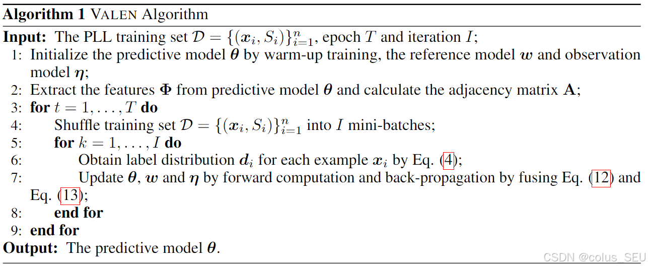
需要训练的有：预测模型（CNN），推理模型（两层 GCN），观测模型（三层MLP）。使用的损失函数包括公式12和公式13.

公式13：通常在全监督学习中，我们最小化预测值与真实标签（One-hot）的交叉熵损失。但在部分标签学习（PLL）中，我们不知道真实标签是哪个，公式通过加权求和来解决这个问题：

\ell(\cdot)：标准的损失函数（如交叉熵），衡量模型预测 f(\boldsymbol{x}_i) 与某个候选标签 \boldsymbol{e}^{y_j} 的距离。

d_i^{y_j} 是标签增强阶段恢复出的潜在概率。公式对 d_i^{y_j} 进行了重归一化，只考虑候选集合 S_i 中的标签，使其和为 1。这意味着我们信任恢复出来的标签分布，用它作为"软标签（Soft Label）"来指导分类器。如果 GCN 认为候选集中某个标签的概率很高，分类器就会重点去拟合这个标签。

Let \widehat{f}V = \min{f \in \mathcal{F}} \widehat{R}V(f) be the empirical risk minimizer and f^\star = \min{f \in \mathcal{F}} R_V(f) be the optimal risk minimizer where R_V(f) is the risk estimator. Besides, we define the function space \mathcal{H}{y_j} for the label y_j \in \mathcal{Y} as \{h: \boldsymbol{x} \mapsto f{y_j}(\boldsymbol{x}) \mid f \in \mathcal{F}\}. Let \mathfrak{R}n\left(\mathcal{H}{y_j}\right) be the expected Rademacher complexity [Bartlett and Mendelson 2002] of \mathcal{H}_{y_j} with sample size n, then we have the following theorem.

Theorem 1 Assume the loss function \ell\left(f(\boldsymbol{x}), \boldsymbol{e}^{y_j}\right) is L-Lipschitz with respect to f(\boldsymbol{x}) (0 < L < \infty) for all y_j \in \mathcal{Y} and upper-bounded by M, i.e., M = \sup_{\boldsymbol{x} \in \mathcal{X}, f \in \mathcal{F}, y_j \in \mathcal{Y}} \ell\left(f(\boldsymbol{x}), \boldsymbol{e}^{y_j}\right). Then, for any \delta > 0, with probability at least 1 - \delta,

R\\left(\\widehat{f}_V\\right) - R\\left(f\^\\star\\right) \\leq 4\\sqrt{2}L \\sum_{j=1}\^{c} \\mathfrak{R}_n\\left(\\mathcal{H}_{y_j}\\right) + M \\sqrt{\\frac{\\log \\frac{2}{\\delta}}{2n}}.

Theorem 1 shows that the empirical risk minimizer f_V converges to the optimal risk minimizer f^\star as n \to \infty and \mathfrak{R}n\left(\mathcal{H}{y_j}\right) \to 0 for all parametric models with a bounded norm.

定理 1 证明了 VALEN 估计器是一致的（Consistent）：只要样本量足够大，通过最小化公式 (13) 中的经验风险，一定能收敛到最优的分类器 f^\star 。

Experiments

Datasets

We adopt four widely used benchmark datasets including MNIST , Fashion-MNIST , Kuzushiji-MNIST, CIFAR-10 , and five datasets from the UCI Machine Learning Repository , including Yeast, Texture, Dermatology, Synthetic Control, and 20Newsgroups.

以上数据集都是小型图像数据集，是有干净标签的，需要处理成部分标签数据集。

We manually corrupt these datasets into partially labeled versions by using a flipping probability \xi_i^{y_j} = P(l_i^{y_j}=1|\hat{l}_i^{y_j}=0, \boldsymbol{x}_i), where \hat{l}_i^{y_j} is the original clean label. To synthesize the instance-dependent candidate labels, we set the flipping probability of each incorrect label corresponding to an example \boldsymbol{x}_i by using the confidence prediction of a clean neural network \hat{\theta} (trained with the original clean labels) with \xi_i^{y_j} = \frac{f_j(\boldsymbol{x}i;\hat{\theta})}{\max{y_j\in\bar{Y}_i}f_j(\boldsymbol{x}_i;\hat{\theta})}, where \bar{Y}_i is the incorrect label set of \boldsymbol{x}_i. The uniform corrupted version adopts the uniform generating procedure to flip the incorrect label into candidate label, where \xi_i^{y_j} = \frac{1}{2}.

该论文使用了两种部分标签生成方案：

FPS (Fliping Probability Strategy)：所有非正确标签以 \xi_i^{y_j} 的概率出现在候选标签集中。要获得该概率，先要有一个在干净数据集上全监督学习训练的神经网络 \hat{\theta}，依据该模型输出的置信度通过公式 \xi_i^{y_j} = \frac{f_j(\boldsymbol{x}i;\hat{\theta})}{\max{y_j\in\bar{Y}_i}f_j(\boldsymbol{x}_i;\hat{\theta})} 得到相应的翻转概率。总的来说，就是该模型预测的概率越高，该非候选标签越有可能出现在候选标签集中。

⚠️这里使用了干净的数据来训练模型，再利用该模型来生成部分标签数据集，其实是受限于没有人工标注的真实部分标签数据集，不得已采用该种方案。其实如果能获得干净数据集的话，直接用来训练模型肯定会更好。当然在实验中这样操作也没有太大的毛病。

UPS (Uniform Probability Strategy) ：所有非正确标签以 \frac{1}{2} 的概率出现在候选标签集中。

In addition, five real-world PLL datasets are adopted, which are collected from several application domains including Lost, Soccer Player and Yahoo! News for automatic face naming from images or videos, MSRCv2 for object classification, and BirdSong for bird song classification. The detailed descriptions of these datasets are provided in Appendix A.3. We run 5 trials on the four benchmark datasets and perform five-fold cross-validation on UCI datasets and real-world PLL datasets. The mean accuracy as well as standard deviation are recorded for all comparing approaches.

这是五个真实部分标签数据集，是小型表格数据集。

Conclusion

In this paper, the problem of partial label learning is studied where a novel approach VALEN is proposed. We for the first time consider the instance-dependent PLL and assume that each partially labeled example is associated with a latent label distribution, which is the essential labeling information and worth being recovered for predictive model training. VALEN recovers the latent label distribution via inferring the true posterior density of the latent label distribution by Dirichlet density parameterized with an inference model and deduce the evidence lower bound for optimization. In addition, VALEN iteratively recovers latent label distributions and trains the predictive model in every epoch. The effectiveness of the proposed approach is validated via comprehensive experiments on both synthesis datasets and real-world PLL datasets.

该论文的核心贡献在于提出了一个 Instance-dependent PLL 的学习范式，通过考虑候选标签集其实是和该样本有关的而不是随机存在的，使得 PLL 问题的更加接近真实情景。其提出的 VALEN 方法通过建模潜在标签分布来解决该问题，建模方式使用的是由一个可训练的 GCN 参数化的狄利克雷分布。笔者认为该论文的亮点在于提出了 ID-PLL，其 VALEN 方法其实效果并不是特别突出，或者说我认为其建模的出发点不够自然，但是其中的数学推导还是颇具亮点的。

✅ 补充知识

一、狄利克雷分布

Dirichlet Distribution 是统计学中一个非常重要的分布。我们从直观理解 、几何意义 、数学定义 以及在机器学习中的作用这四个层面介绍。

1. 直观理解：它是"概率分布的分布"

要理解狄利克雷分布，最好的方式是把它看作**"生产骰子的工厂"**。

普通的骰子（多项分布）： 掷一个骰子，结果可能是 1 到 6 点。描述这个骰子的性质需要一个概率向量，例如公平骰子是 \boldsymbol{p} = [1/6, 1/6, \dots, 1/6]。
狄利克雷分布： 想象一个工厂生产各种各样的骰子。
- 有的骰子是公平的。
- 有的骰子灌了铅，总是掷出 6。
- 有的骰子偏向于 1 和 2。
狄利克雷分布就是描述这个工厂生产出"某种特定概率特征的骰子"的概率。 换句话说，它是从所有可能的概率分布（单纯形）中进行采样的分布。因此，它常被称为"分布的分布"。

2. 几何意义：单纯形 (Simplex)

狄利克雷分布是定义在单纯形上的。

什么是单纯形？

如果我们要描述 3 个类别的概率（例如石头、剪刀、布），这三个概率必须满足 p_1 + p_2 + p_3 = 1 且 p_i \ge 0。在三维空间中，满足这个条件的点构成了一个三角形（二维平面）。这个三角形就是单纯形。
参数 \boldsymbol{\alpha} 的控制作用：

狄利克雷分布由参数向量 \boldsymbol{\alpha} = [\alpha_1, \alpha_2, \dots, \alpha_K] 控制。这个参数决定了概率密度在单纯形上的形状：
1. 稀疏分布 (\alpha_i < 1)： 如论文中的 \epsilon。概率密度聚集在单纯形的顶点（角）。
  - 意义： 采样的分布倾向于"极端"。比如，我们要么非常确定是类别 A，要么非常确定是类别 B，很少出现模棱两可的情况。
2. 均匀分布 (\alpha_i = 1)： 概率密度在单纯形上是均匀的。
  - 意义： 所有可能的概率分布出现的概率都一样。
3. 集中分布 (\alpha_i > 1)： 概率密度聚集在单纯形的中心。
  - 意义： 采样的分布倾向于"平均"。比如每个类别的概率都接近 1/K。

3. 数学定义

假设我们有一个 K 维的随机向量 \boldsymbol{x} = (x_1, \dots, x_K)，如果它服从参数为 \boldsymbol{\alpha} 的狄利克雷分布，记作 \boldsymbol{x} \sim Dir(\boldsymbol{\alpha})，其概率密度函数（PDF）为：

\\color{blue} f(\\boldsymbol{x}; \\boldsymbol{\\alpha}) = \\frac{1}{B(\\boldsymbol{\\alpha})} \\prod_{i=1}\^{K} x_i\^{\\alpha_i - 1}

其中：

\boldsymbol{x} 的约束：\sum_{i=1}^K x_i = 1, \quad x_i \ge 0。
B(\boldsymbol{\alpha})：是归一化常数，称为多变量贝塔函数（Multivariate Beta Function）。它的定义与伽马函数（Gamma Function, Γ）有关：
$B(\\boldsymbol{\\alpha}) = \\frac{\\prod_{i=1}\^K \\Gamma(\\alpha_i)}{\\Gamma(\\sum_{i=1}\^K \\alpha_i)}$

论文的公式 (7) 中直接应用了这个密度函数。公式 (7) 计算了 \mathrm{KL}(q||p)，其中的 log~\Gamma(\cdot) 和 \psi(\cdot)（Digamma function，即伽马函数对数的导数）正是对上述概率密度函数取对数并求期望后产生的项。

4. 为什么机器学习偏爱它？

狄利克雷分布在贝叶斯推断和机器学习中有两个核心优势：

A. 共轭先验 (Conjugate Prior)

这是最重要的数学性质。

场景：如果你有一个多分类问题（服从多项分布，Multinomial），你想估计每个类的概率。
便利性 ：如果你假设这些概率的先验分布 是狄利克雷分布，那么根据贝叶斯公式计算出来的后验分布 （Posterior）依然是一个狄利克雷分布。
论文中的体现：这就是为什么论文第 2.3 节可以用变分推断（Variational Inference）推导出一个解析解（Closed-form solution）。如果选了高斯分布作为先验，对应多项分布的似然函数，后验分布会变得极其复杂，无法直接计算。

B. 归纳偏置 (Inductive Bias) 的注入

通过调节 \alpha，我们可以轻松地把人类的先验知识（Inductive Bias）注入模型。论文中作者通过设置 \alpha < 1，明确告诉模型："虽然这是一个部分标签学习问题，但我相信对于大多数样本，真实的标签分布应该是尖锐的（Sharp），请往这个方向优化。"

二、图卷积网络

简单来说，GCN 就是一种让数据样本"互相交流、交换信息"的神经网络。

1. 为什么要用图（Graph）？

在传统的神经网络（如处理图像的 CNN）中，数据是排列整齐的网格（Grid）。比如像素点，每个点都有固定的上下左右邻居。

但在 VALEN 这篇论文的场景中，数据是非欧几里得结构的：

我们有一堆样本（图片），它们之间并没有固定的空间位置关系。
但是，有些图片长得很像（特征相似），我们可以把它们连起来。
节点 (Node)：每一个圆圈代表一张图片（或者说一个样本 x_i）。
边 (Edge)：如果两张图片特征很像（比如都是圆形的物体），它们之间就有一条线相连。这对应论文公式 (3) 中构建的 a_{ij} 。

2. GCN 的核心思想：消息传递 (Message Passing)

理解 GCN 最好的方式是把它想象成社交网络中的"八卦传播"。

核心假设（同质性 Homophily）： "物以类聚，人以群分"。如果你的朋友都很聪明，那你大概率也挺聪明；如果你的邻居都是"猫"的图片，那你大概率也是"猫"。

GCN 做的事情分两步：

聚合（Aggregate / Gather）：

每个节点都会向它的邻居"打听消息"。
- 例子：节点 A 问它的邻居 B 和 C："你们是什么特征？你们觉得这一类的标签分布是什么？"
- 对应论文 ：这就是矩阵 \tilde{\mathbf{A}} 乘法的作用。在数学上，乘以邻接矩阵 \mathbf{A} 等同于把所有邻居的特征值**加和（Sum）**起来。
更新（Update）：

节点 A 收到邻居 B 和 C 的信息后，结合自己原本的信息，经过一个神经网络层（权重变换），更新自己的状态。
- 结果：节点 A 的特征变得更丰富了，它不仅包含了自己的视觉信息，还融合了邻居的信息。

3. 对照论文公式详解

论文中的 GCN 公式就是上述过程的数学写法：

\\text{GCN}(\\mathbf{Z}) = \\underbrace{\\tilde{\\mathbf{A}}}_{\\text{邻居信息聚合}} \\quad \\text{ReLU}\\left( \\underbrace{\\tilde{\\mathbf{A}}}_{\\text{邻居信息聚合}} \\mathbf{Z} \\underbrace{\\mathbf{W}_0}_{\\text{特征变换}} \\right) \\mathbf{W}_1

VALEN 里的 GCN 就是一个混合器 。它把一张图片自己的特征 和它邻居（相似图片）的特征混合在一起，大家互相"对答案"，从而把原本模糊不清的候选标签，提纯成一个清晰的、可信度高的概率分布（狄利克雷分布参数）。