文章目录
-
- 一、序列模型的具体示例
- 二、循环神经网络模型
-
- [2.1 普通神经网络](#2.1 普通神经网络)
- [2.2 循环神经网络模型](#2.2 循环神经网络模型)
-
- [2.2.1 正向传播](#2.2.1 正向传播)
- [2.2.2 反向传播](#2.2.2 反向传播)
- [2.2.3 构建循环神经网络代码示例](#2.2.3 构建循环神经网络代码示例)
-
- [2.2.3.1 定义循环神经网络](#2.2.3.1 定义循环神经网络)
- [2.2.3.2 单个示例向前传播](#2.2.3.2 单个示例向前传播)
- [2.2.3.3 循环神经网络向前传播](#2.2.3.3 循环神经网络向前传播)
- [2.2.3.4 向后传播](#2.2.3.4 向后传播)
- [2.3 修改的循环神经网络](#2.3 修改的循环神经网络)
- 三、语言模型和序列生成
-
- [3.1 搭建语言模型](#3.1 搭建语言模型)
- [3.2 对新序列进行抽样](#3.2 对新序列进行抽样)
- 四、RNNs的梯度消失
-
- [4.1 GRU(Gated Recurrent Unit)门控循环单元](#4.1 GRU(Gated Recurrent Unit)门控循环单元)
- [4.2 长短期记忆单元(LSTM)](#4.2 长短期记忆单元(LSTM))
-
- [4.2.1 长短期记忆单元LSTM原理](#4.2.1 长短期记忆单元LSTM原理)
- [4.2.2 构建一个长短期记忆网络](#4.2.2 构建一个长短期记忆网络)
-
- [4.2.2.1 遗忘门](#4.2.2.1 遗忘门)
- [4.2.2.2 更新门](#4.2.2.2 更新门)
- [4.2.2.3 输出门](#4.2.2.3 输出门)
- [4.2.2.4 单个时间节点的LSTM向前传播](#4.2.2.4 单个时间节点的LSTM向前传播)
- [4.2.2.5 LSTM向前传播代码示例](#4.2.2.5 LSTM向前传播代码示例)
- [4.2.2.6 向后传播](#4.2.2.6 向后传播)
- 五、双向递归神经网络(BRNN)
- 六、深度RNNs
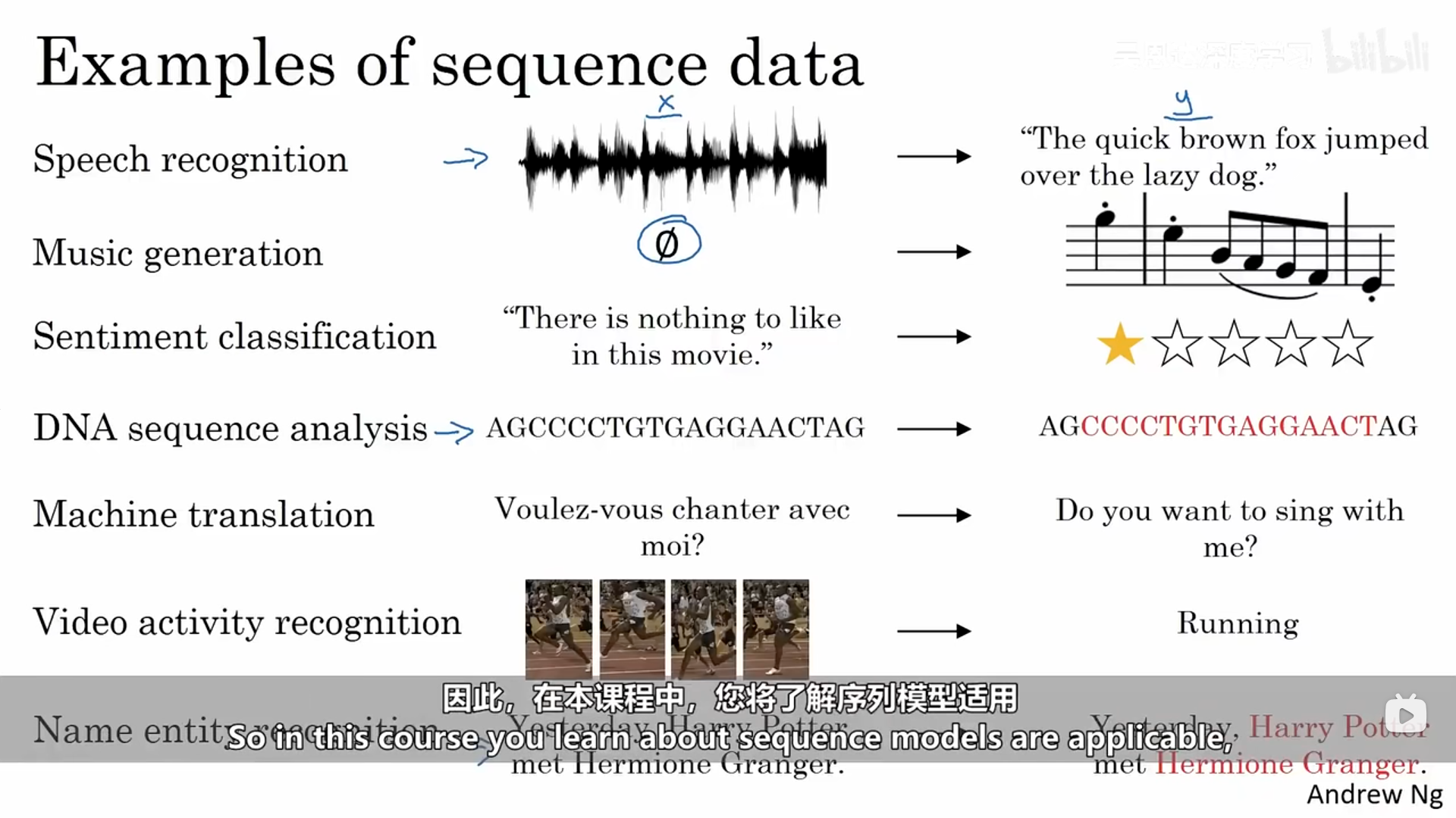
序列模型常常在下列领域得到应用,它们通常是有监督学习,X、Y都为序列数据,或者只有某一个是序列数据。
一、序列模型的具体示例
下面是一个关于识别一个句子序列中人名的示例:输入的数据是一个句子,输出是句子对应位置是否是人名(1/0)。
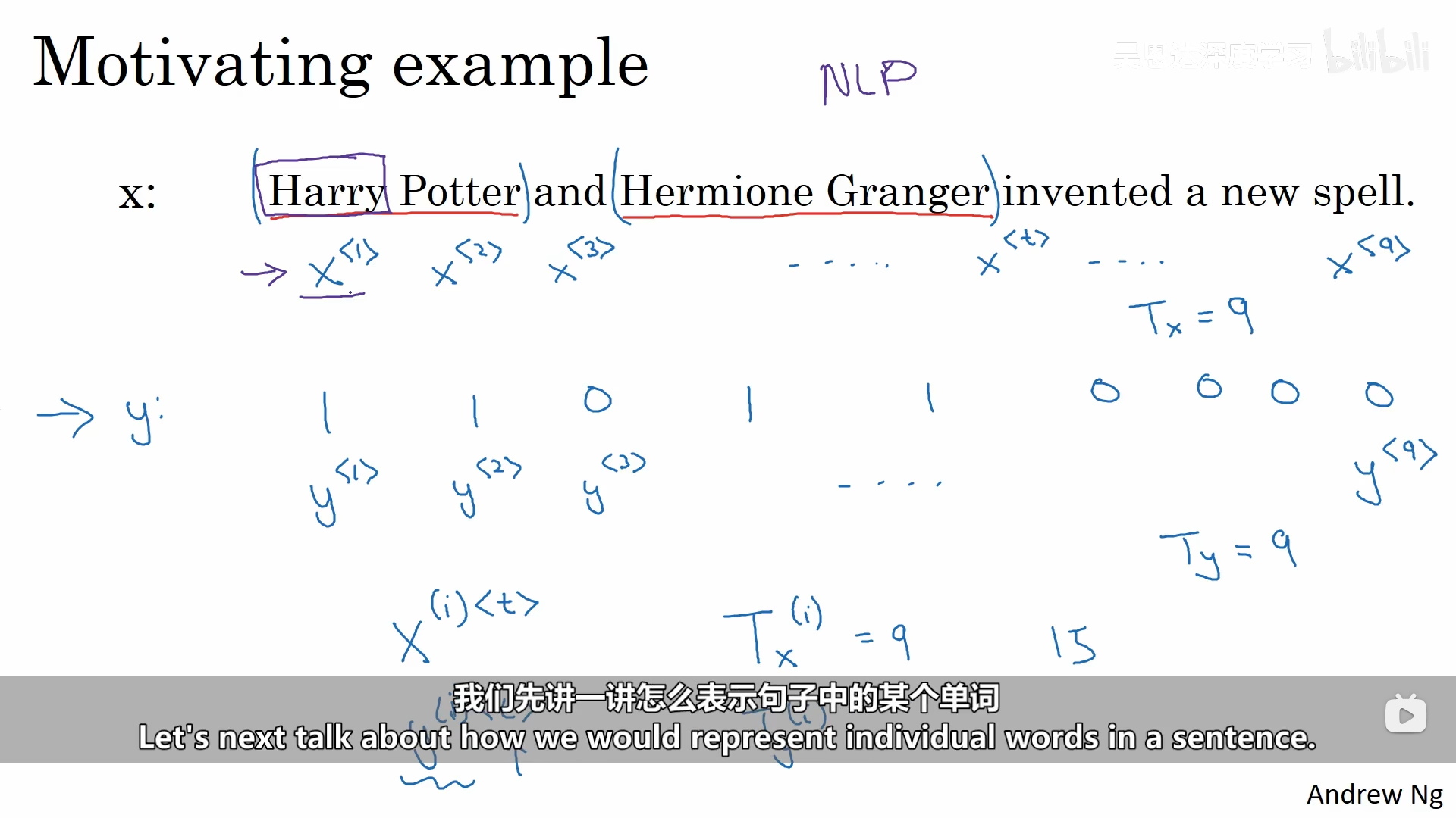
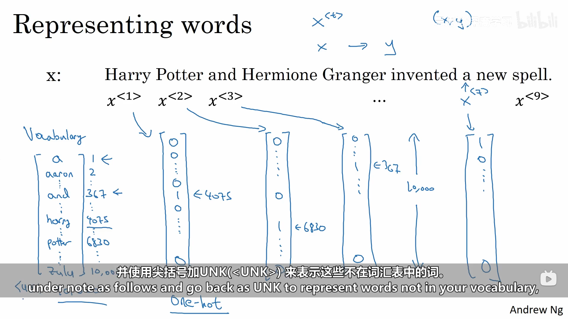
我们如何描述句子中的每一个词呢,这个过程需要使用到自然语言处理。首先我们需要先有一个词典,我们可以根据词典对句子中的每一个单词进行独热编码,每一个单词就是一个维数为词典大小的向量。
二、循环神经网络模型
2.1 普通神经网络
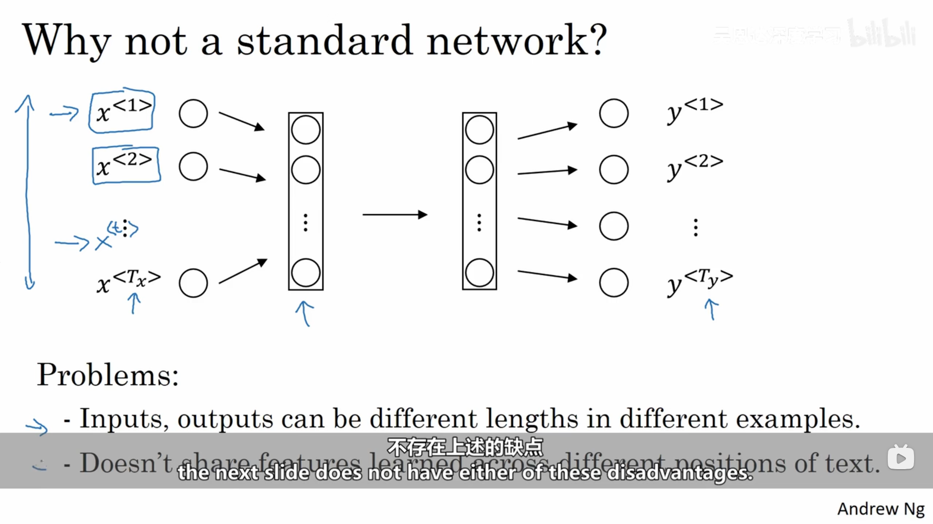
我们可以对上面的数据使用普通的神经网络,但是回存在两个问题:第一个问题每一个样本的输入和输出的大小不同;第二个问题是它并不会共享那些从不同文本位置学到的特征。不仅如此,这样也会导致网络的参数量巨大,计算成本太高。
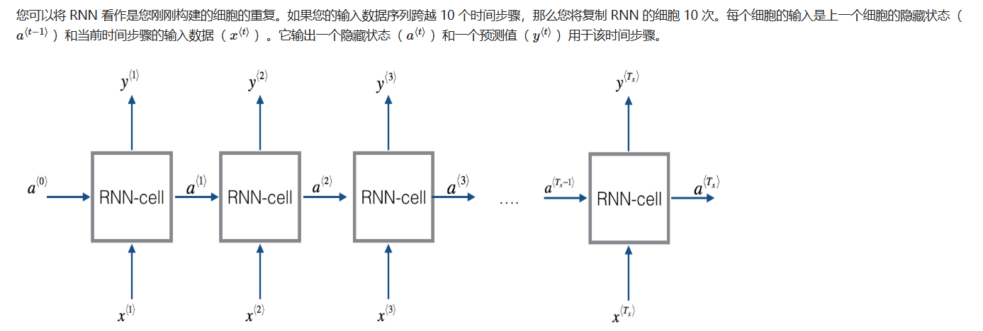
2.2 循环神经网络模型
由于它们具有"记忆",所以循环神经网络(RNN)在自然语言处理和其他序列任务中非常有效。它们可以一次读取一个输入(例如单词),并且通过隐藏层的激活值记住一些信息/上下文,这些激活值从一个时间步传递到下一个时间步。这使得单向 RNN 能够从过去获取信息,以处理后续输入。双向 RNN 可以获取过去和未来的上下文。
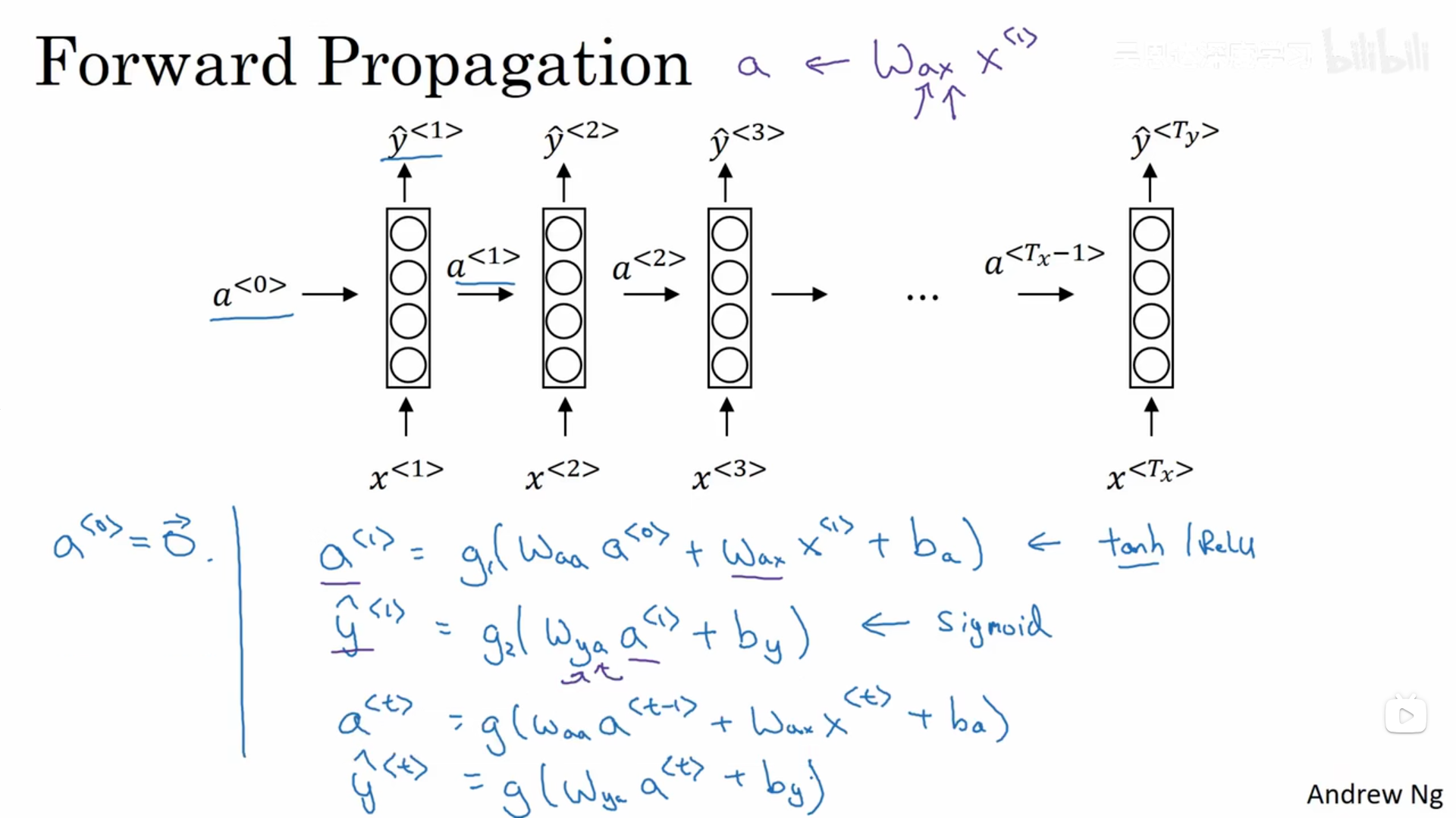
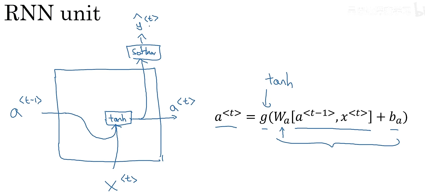
2.2.1 正向传播
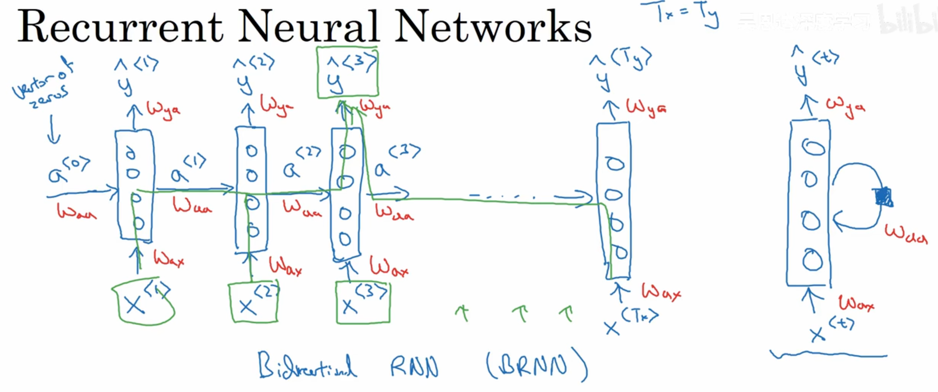
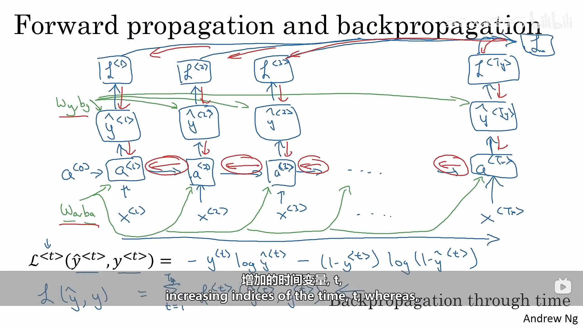
而循环神经网络是怎么做的呢?首先取出句子中的第一个单词,输入到神经网络中去,进行预测输出,判断这个单词是都是人名的一部分,接着继续取出第二个单词,这里我们不仅仅通过这个单词作为输入,还会将第一步的计算结果也作为第二步的输入信息一起输入进去(第一步的激活数值会传递到第二步)。以此类推。在第一步的时候,往往也会有人造的激活值(常常是全0)作为输入传递给它.循环神经网络是从左到右扫描数据,每一步它所用的参数是共享的。这也意味着循环神经网络有一个缺点,它所共享的信息都是来自于之前的,而后面的信息没有利用到。
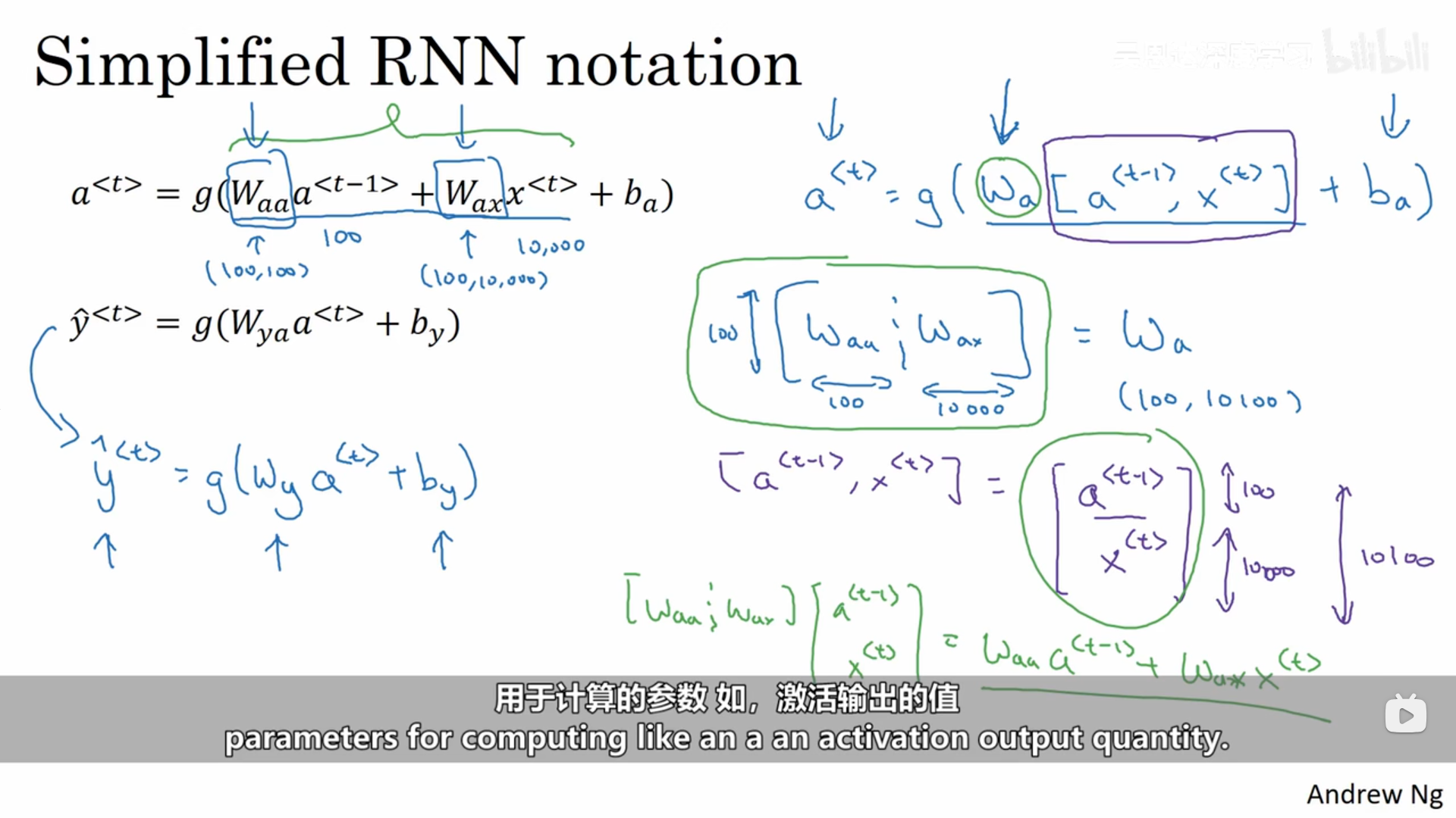
具体的计算方式(正向传播)如下:
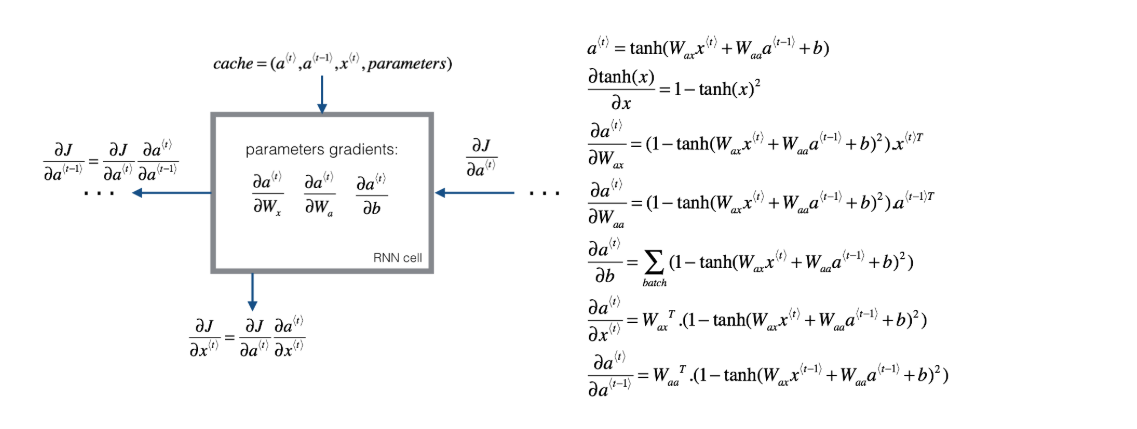
2.2.2 反向传播
下面图像中的蓝色箭头表示了循环神经网络的正向传播,红色箭头则代表循环神经网络的反向传播。
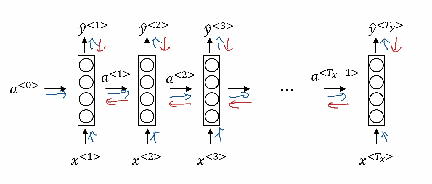
下图展示了循环神经网络反向传播的过程:
上面所讲述的结构都是基于输入和输出的长度是相等的情况,下面继续展示更广泛的RNN体系结构。
2.2.3 构建循环神经网络代码示例
2.2.3.1 定义循环神经网络
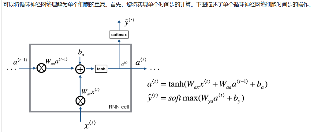
2.2.3.2 单个示例向前传播
plain
# GRADED FUNCTION: rnn_cell_forward
def rnn_cell_forward(xt, a_prev, parameters):
"""
Implements a single forward step of the RNN-cell as described in Figure (2)
Arguments:
xt -- your input data at timestep "t", numpy array of shape (n_x, m).
a_prev -- Hidden state at timestep "t-1", numpy array of shape (n_a, m)
parameters -- python dictionary containing:
Wax -- Weight matrix multiplying the input, numpy array of shape (n_a, n_x)
Waa -- Weight matrix multiplying the hidden state, numpy array of shape (n_a, n_a)
Wya -- Weight matrix relating the hidden-state to the output, numpy array of shape (n_y, n_a)
ba -- Bias, numpy array of shape (n_a, 1)
by -- Bias relating the hidden-state to the output, numpy array of shape (n_y, 1)
Returns:
a_next -- next hidden state, of shape (n_a, m)
yt_pred -- prediction at timestep "t", numpy array of shape (n_y, m)
cache -- tuple of values needed for the backward pass, contains (a_next, a_prev, xt, parameters)
"""
# Retrieve parameters from "parameters"
Wax = parameters["Wax"]
Waa = parameters["Waa"]
Wya = parameters["Wya"]
ba = parameters["ba"]
by = parameters["by"]
### START CODE HERE ### (≈2 lines)
# compute next activation state using the formula given above
a_next = np.tanh(np.dot(Wax, xt) + np.dot(Waa, a_prev) + ba) # 计算下一时刻隐藏状态:tanh(Wax·xt + Waa·a_prev + ba),其中ba会按列广播到(m)个样本
# compute output of the current cell using the formula given above
yt_pred = softmax(np.dot(Wya, a_next) + by) # 计算当前时刻输出概率:softmax(Wya·a_next + by),by同样会对(m)个样本广播
### END CODE HERE ###
# store values you need for backward propagation in cache
cache = (a_next, a_prev, xt, parameters)
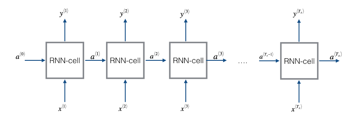
return a_next, yt_pred, cache2.2.3.3 循环神经网络向前传播
plain
# GRADED FUNCTION: rnn_forward

def rnn_forward(x, a0, parameters):
    """
    Implement the forward propagation of the recurrent neural network described in Figure (3).

    Arguments:
    x -- Input data for every time-step, of shape (n_x, m, T_x).
    a0 -- Initial hidden state, of shape (n_a, m)
    parameters -- python dictionary containing:
                        Waa -- Weight matrix multiplying the hidden state, numpy array of shape (n_a, n_a)
                        Wax -- Weight matrix multiplying the input, numpy array of shape (n_a, n_x)
                        Wya -- Weight matrix relating the hidden-state to the output, numpy array of shape (n_y, n_a)
                        ba --  Bias numpy array of shape (n_a, 1)
                        by -- Bias relating the hidden-state to the output, numpy array of shape (n_y, 1)

    Returns:
    a -- Hidden states for every time-step, numpy array of shape (n_a, m, T_x)
    y_pred -- Predictions for every time-step, numpy array of shape (n_y, m, T_x)
    caches -- tuple of values needed for the backward pass, contains (list of caches, x)
    """

    # Initialize "caches" which will contain the list of all caches
    caches = []

    # Retrieve dimensions from shapes of x and Wy
    n_x, m, T_x = x.shape
    n_y, n_a = parameters["Wya"].shape

    ### START CODE HERE ###

    # initialize "a" and "y" with zeros (≈2 lines)
    a = np.zeros((n_a, m, T_x))                 # 初始化所有时间步的隐藏状态张量 a,形状 (n_a, m, T_x)
    y_pred = np.zeros((n_y, m, T_x))            # 初始化所有时间步的预测输出张量 y_pred,形状 (n_y, m, T_x)

    # Initialize a_next (≈1 line)
    a_next = a0                                  # 将下一隐藏状态初始化为初始隐藏状态 a0,形状 (n_a, m)

    # loop over all time-steps
    for t in range(T_x):                         # 遍历每一个时间步 t = 0..T_x-1

        # Update next hidden state, compute the prediction, get the cache (≈1 line)
        a_next, yt_pred, cache = rnn_cell_forward(x[:, :, t], a_next, parameters)  # 用当前输入x_t和上一隐藏状态计算新隐藏状态a_next与当前输出yt_pred,并拿到cache

        # Save the value of the new "next" hidden state in a (≈1 line)
        a[:, :, t] = a_next                      # 把当前时间步的隐藏状态存入 a 的第 t 个切片

        # Save the value of the prediction in y (≈1 line)
        y_pred[:, :, t] = yt_pred                # 把当前时间步的预测结果存入 y_pred 的第 t 个切片

        # Append "cache" to "caches" (≈1 line)
        caches.append(cache)                     # 将当前时间步的cache追加到caches列表,供反向传播使用

    ### END CODE HERE ###


    # store values needed for backward propagation in cache
    caches = (caches, x)

    return a, y_pred, caches
2.2.3.4 向后传播
plain
def rnn_cell_backward(da_next, cache):
    """
    Implements the backward pass for the RNN-cell (single time-step).

    Arguments:
    da_next -- Gradient of loss with respect to next hidden state
    cache -- python dictionary containing useful values (output of rnn_step_forward())

    Returns:
    gradients -- python dictionary containing:
                        dx -- Gradients of input data, of shape (n_x, m)
                        da_prev -- Gradients of previous hidden state, of shape (n_a, m)
                        dWax -- Gradients of input-to-hidden weights, of shape (n_a, n_x)
                        dWaa -- Gradients of hidden-to-hidden weights, of shape (n_a, n_a)
                        dba -- Gradients of bias vector, of shape (n_a, 1)
    """

    # Retrieve values from cache
    (a_next, a_prev, xt, parameters) = cache

    # Retrieve values from parameters
    Wax = parameters["Wax"]
    Waa = parameters["Waa"]
    Wya = parameters["Wya"]
    ba = parameters["ba"]
    by = parameters["by"]

    ### START CODE HERE ###
    # compute the gradient of tanh with respect to a_next (≈1 line)
    dtanh = (1 - np.square(a_next)) * da_next                 # tanh导数:dZ = (1 - a_next^2) ⊙ da_next,其中Z=Wax·xt+Waa·a_prev+ba

    # compute the gradient of the loss with respect to Wax (≈2 lines)
    dxt = np.dot(Wax.T, dtanh)                                # 对输入xt的梯度:dxt = Wax^T · dZ,形状(n_x, m)
    dWax = np.dot(dtanh, xt.T)                                # 对Wax的梯度:dWax = dZ · xt^T,形状(n_a, n_x)

    # compute the gradient with respect to Waa (≈2 lines)
    da_prev = np.dot(Waa.T, dtanh)                            # 对上一隐藏状态a_prev的梯度:da_prev = Waa^T · dZ,形状(n_a, m)
    dWaa = np.dot(dtanh, a_prev.T)                            # 对Waa的梯度:dWaa = dZ · a_prev^T,形状(n_a, n_a)

    # compute the gradient with respect to b (≈1 line)
    dba = np.sum(dtanh, axis=1, keepdims=True)                # 对偏置ba的梯度:对batch维m求和,保持形状(n_a, 1)
    ### END CODE HERE ###


    # Store the gradients in a python dictionary
    gradients = {"dxt": dxt, "da_prev": da_prev, "dWax": dWax, "dWaa": dWaa, "dba": dba}

    return gradients
plain
def rnn_backward(da, caches):
    """
    Implement the backward pass for a RNN over an entire sequence of input data.

    Arguments:
    da -- Upstream gradients of all hidden states, of shape (n_a, m, T_x)
    caches -- tuple containing information from the forward pass (rnn_forward)

    Returns:
    gradients -- python dictionary containing:
                        dx -- Gradient w.r.t. the input data, numpy-array of shape (n_x, m, T_x)
                        da0 -- Gradient w.r.t the initial hidden state, numpy-array of shape (n_a, m)
                        dWax -- Gradient w.r.t the input's weight matrix, numpy-array of shape (n_a, n_x)
                        dWaa -- Gradient w.r.t the hidden state's weight matrix, numpy-arrayof shape (n_a, n_a)
                        dba -- Gradient w.r.t the bias, of shape (n_a, 1)
    """

    ### START CODE HERE ###

    # Retrieve values from the first cache (t=1) of caches (≈2 lines)
    (caches_list, x) = caches                                  # 解包caches:caches_list是每个时间步的cache列表,x是原始输入序列
    (a1, a0, x1, parameters) = caches_list[0]                  # 取第0个时间步的cache来拿到x1/parameters等(模板里叫t=1但这里是索引0)

    # Retrieve dimensions from da's and x1's shapes (≈2 lines)
    n_a, m, T_x = da.shape                                     # 从da得到隐藏维度n_a、样本数m、时间步数T_x
    n_x, m = x1.shape                                          # 从x1得到输入维度n_x以及样本数m(与上面m一致)

    # initialize the gradients with the right sizes (≈6 lines)
    dx = np.zeros((n_x, m, T_x))                               # 初始化对输入序列x的梯度dx,形状(n_x, m, T_x)
    dWax = np.zeros((n_a, n_x))                                # 初始化对Wax的梯度累加器
    dWaa = np.zeros((n_a, n_a))                                # 初始化对Waa的梯度累加器
    dba = np.zeros((n_a, 1))                                   # 初始化对偏置ba的梯度累加器
    da0 = np.zeros((n_a, m))                                   # 初始化对初始隐藏状态a0的梯度(最后会赋值)
    da_prev = np.zeros((n_a, m))                               # 初始化来自"未来时间步"的隐藏状态梯度(t+1传回来的)

    # Loop through all the time steps
    for t in reversed(range(T_x)):                             # 按时间逆序遍历:T_x-1 -> 0

        # Compute gradients at time step t. Choose wisely the "da_next" and the "cache" to use in the backward propagation step. (≈1 line)
        gradients_t = rnn_cell_backward(da[:, :, t] + da_prev, caches_list[t])  # 当前时刻的da_next = 上游da_t + 来自未来的da_prev,然后用对应cache做单步反传

        # Retrieve derivatives from gradients (≈ 1 line)
        dxt, da_prev, dWaxt, dWaat, dbat = gradients_t["dxt"], gradients_t["da_prev"], gradients_t["dWax"], gradients_t["dWaa"], gradients_t["dba"]  # 取出单步反传得到的各项梯度

        # Increment global derivatives w.r.t parameters by adding their derivative at time-step t (≈4 lines)
        dx[:, :, t] = dxt                                      # 将当前时间步对输入的梯度写入dx的第t个切片
        dWax += dWaxt                                          # 累加每个时间步对Wax的梯度
        dWaa += dWaat                                          # 累加每个时间步对Waa的梯度
        dba += dbat                                            # 累加每个时间步对ba的梯度

    # Set da0 to the gradient of a which has been backpropagated through all time-steps (≈1 line)
    da0 = da_prev                                              # 反传结束后,da_prev就是对初始隐藏状态a0的梯度
    ### END CODE HERE ###


    # Store the gradients in a python dictionary
    gradients = {"dx": dx, "da0": da0, "dWax": dWax, "dWaa": dWaa,"dba": dba}

    return gradients
2.3 修改的循环神经网络
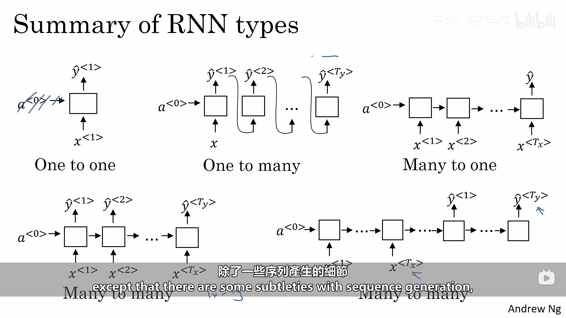
在实际应用中,输入和输出的长度不都是相同,为了解决这类问题,我们需要对基本的循环神经网络结构进行修改。我们上面所讲述的是多对多的情况,即输入和输出都是多个,并且它们相等,以此类推,我们也存在一对一、一对多(音乐创作)、多对多(输入和输出的长度不同、翻译器)、多对一(情感分析)的情况。
三、语言模型和序列生成
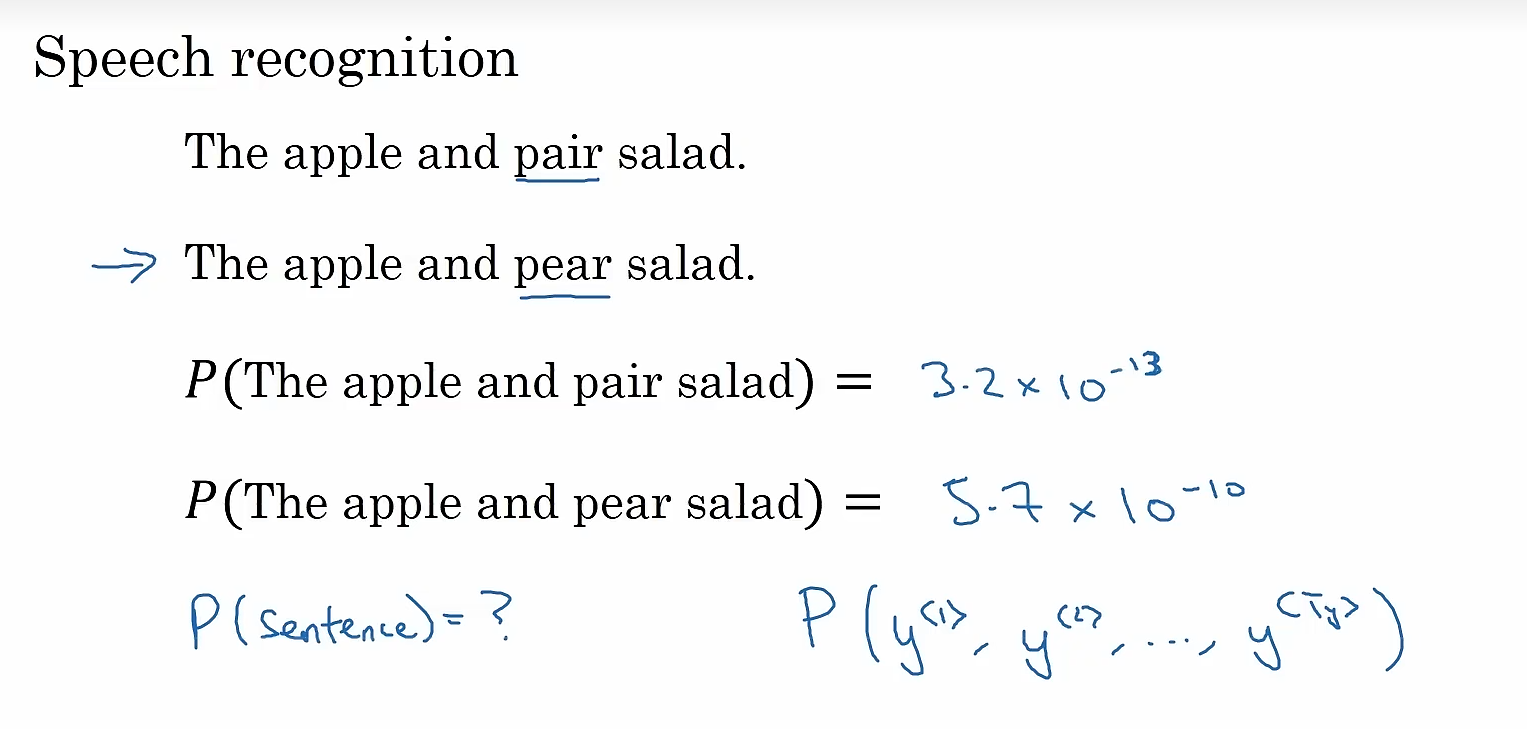
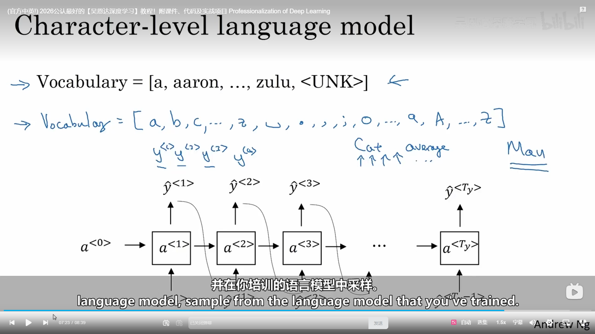
3.1 搭建语言模型
语言模型的工作是:输入一个句子,语言模型需要估计特定单词序列的概率。
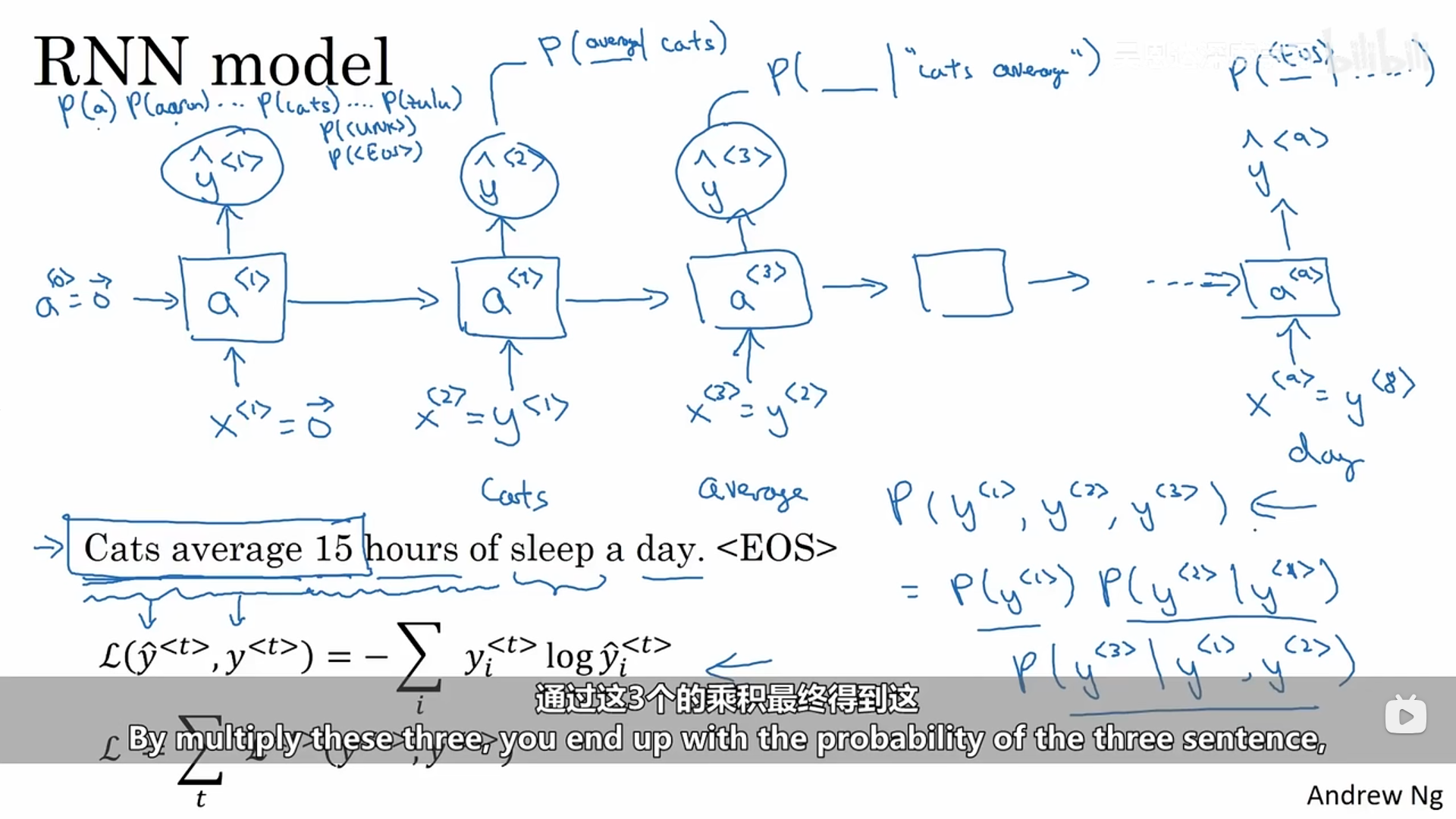
如何使用RNN构建一个语言模型呢?首先我们需要由一个语料库构成的训练集(大体量或者海量英语语句构成的英语文本集合),我们需要对训练集里面的句子进行标记,从而得到一个单词表,然后将各个单词映射到一个一位有效矢量,将对应索引值的矢量元素置一,在句子的结尾会加一个叫做EOS的标记,作为定位的结束。当训练集中有一些单词不在单词表中应该怎么办呢?这种情况下我们可以把Mau用一个全局唯一的标记代替,叫做UNK,表示未知单词。
第一步是使用softmax尝试预测单词表中每个单词的概率(是一个词典大小维数的向量),在进行下一步预测时,我们会告诉它上一步的正确答案。简单来说,每一步预测都是在预测当前位置单词表中所有单词的分布概率。
3.2 对新序列进行抽样
按照3.1所说的方式,训练完成之后,我们可以采集一些新的序列来测试模型学习到了什么。
我们已经知道了在向前传播的过程中我们逐渐预测了每一个位置上单词表中的单词的概率,接下来我们需要做的就是采样,根据概率进行采样,就会采集到我们预测的句子。
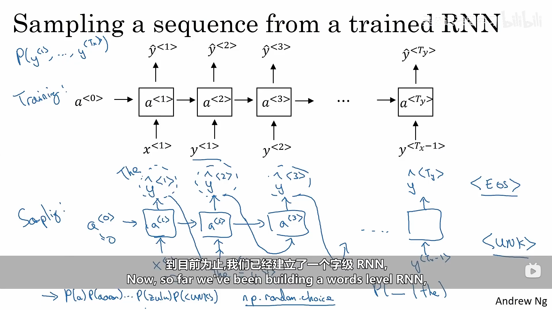
上面成功建立了一个词级的语言模型,与此同时我们也可以建立字符级的语言模型,只是序列就变得更长了。
四、RNNs的梯度消失
在语言模型中,我们从左到右进行正向传播,然后从右到左进行反向传播是非常困难的,因为与深度网络一样,当我们的训练集达到一定数量时,循环神经网络的层数也会增加,常常面临着梯度消失的问题,错误的输出往往会影响到前期的计算,即循环神经网络不擅长捕捉远程依赖关系。
4.1 GRU(Gated Recurrent Unit)门控循环单元
它修改了循环神经网络的隐藏层,从而更好地捕捉长距离的关系,同时有助于减轻梯度消失的问题。
RNN的激活单元可视化如下:
门控循环单元中有一个记忆单元,它提供一些内存来记东西,在时间t,记忆单元会存有一些对应t的c值,GRU单位实际上会输出一个与时间t的c值相等的激活值a。还有一个控制门叫做gama,它代表着要更新的门,这是一个介于0和1之间的值,控制门决定我们是否要更新记忆单元。
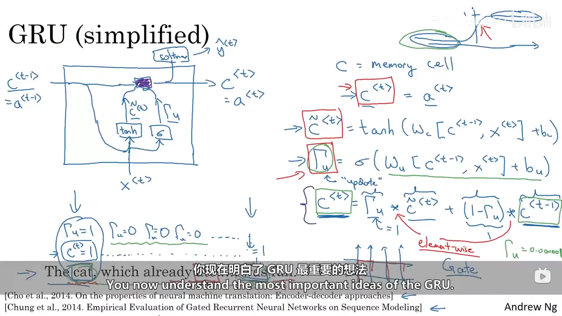
整理之后的公式如下:
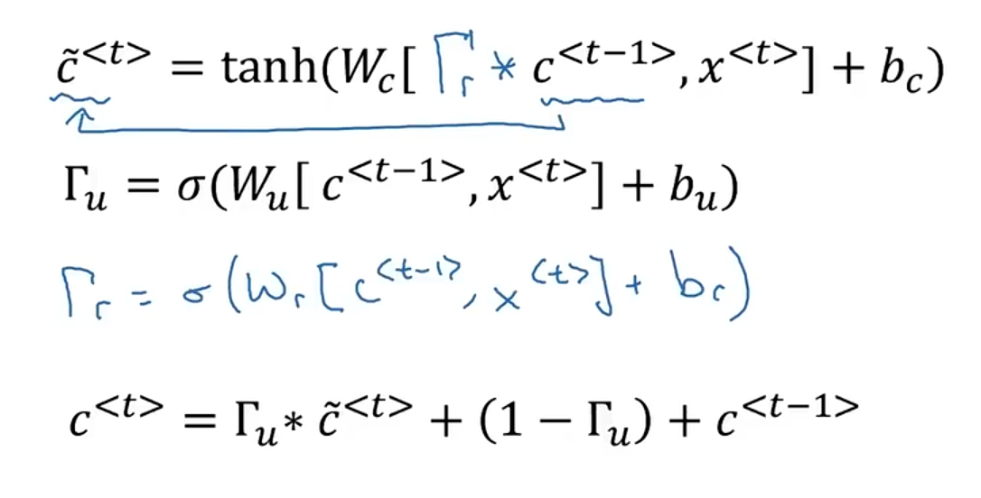
4.2 长短期记忆单元(LSTM)
4.2.1 长短期记忆单元LSTM原理
长短期记忆不再使用相关性门,也不再使用一个控制门,而是使用一个控制门和一个遗忘门。
计算的基本公式如下:
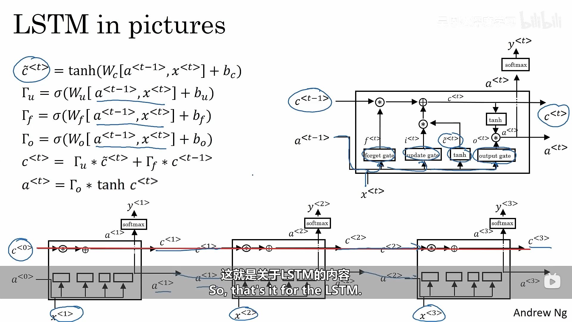
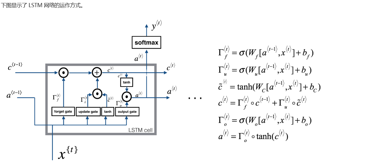
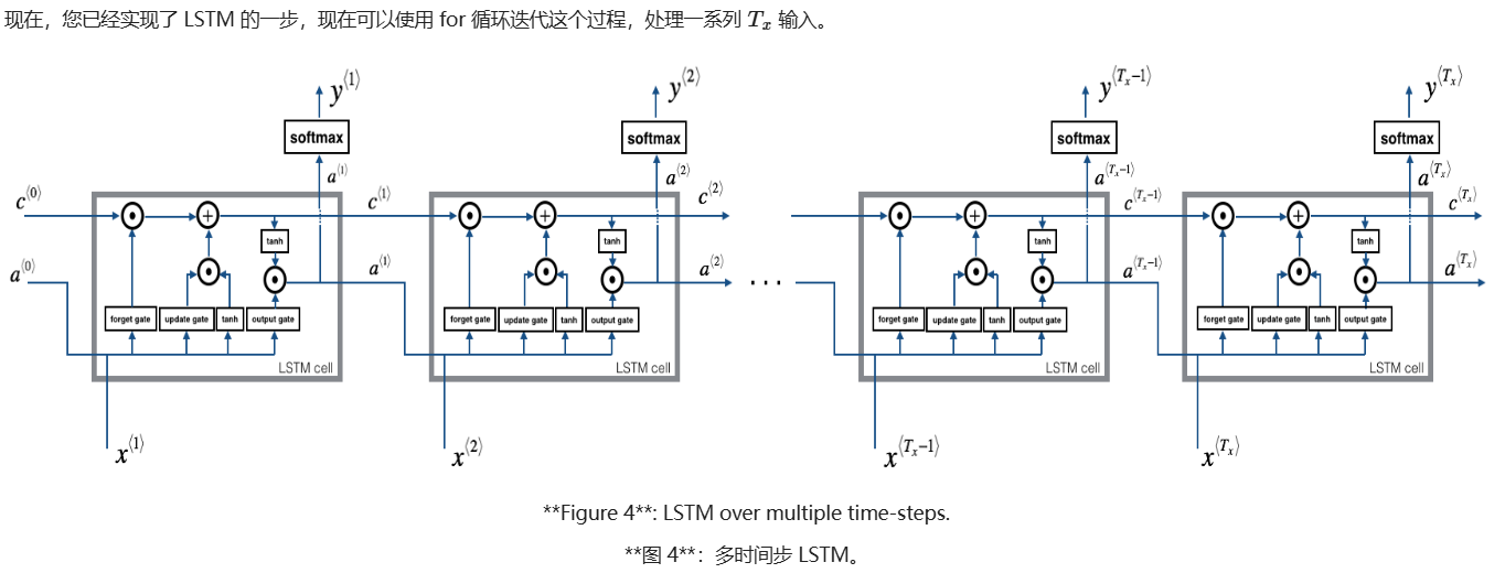
4.2.2 构建一个长短期记忆网络
LSTM 模型,该模型在处理消失梯度方面表现更好。 LSTM 将能够更好地记住信息,并将其保存在许多时间步中。
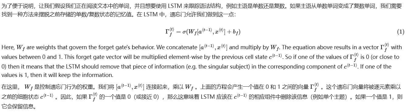
4.2.2.1 遗忘门
4.2.2.2 更新门
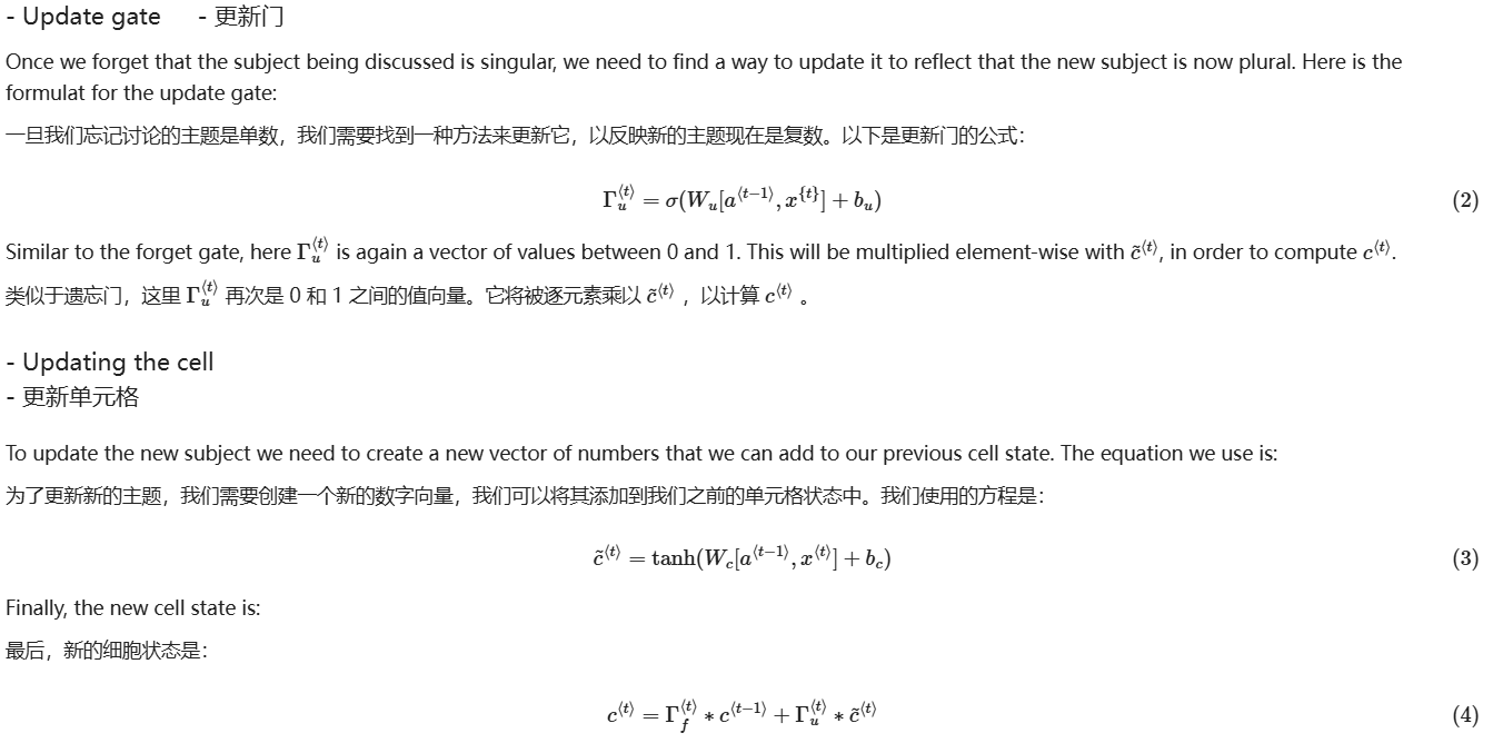
4.2.2.3 输出门
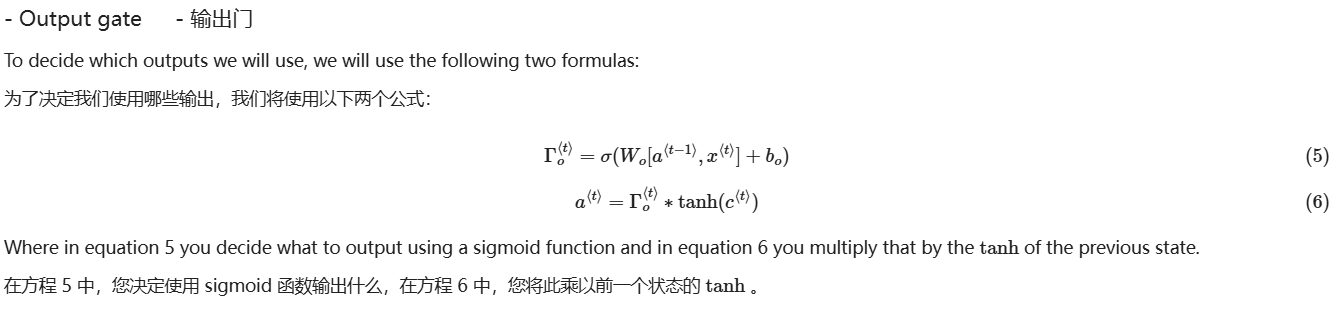
4.2.2.4 单个时间节点的LSTM向前传播
在普通的循环神经网络中使用LSTM长短期记忆网络,某一个时间节点的向前传播代码示例如下:
plain
# GRADED FUNCTION: lstm_cell_forward

def lstm_cell_forward(xt, a_prev, c_prev, parameters):
    """
    Implement a single forward step of the LSTM-cell as described in Figure (4)

    Arguments:
    xt -- your input data at timestep "t", numpy array of shape (n_x, m).
    a_prev -- Hidden state at timestep "t-1", numpy array of shape (n_a, m)
    c_prev -- Memory state at timestep "t-1", numpy array of shape (n_a, m)
    parameters -- python dictionary containing:
                        Wf -- Weight matrix of the forget gate, numpy array of shape (n_a, n_a + n_x)
                        bf -- Bias of the forget gate, numpy array of shape (n_a, 1)
                        Wi -- Weight matrix of the save gate, numpy array of shape (n_a, n_a + n_x)
                        bi -- Bias of the save gate, numpy array of shape (n_a, 1)
                        Wc -- Weight matrix of the first "tanh", numpy array of shape (n_a, n_a + n_x)
                        bc --  Bias of the first "tanh", numpy array of shape (n_a, 1)
                        Wo -- Weight matrix of the focus gate, numpy array of shape (n_a, n_a + n_x)
                        bo --  Bias of the focus gate, numpy array of shape (n_a, 1)
                        Wy -- Weight matrix relating the hidden-state to the output, numpy array of shape (n_y, n_a)
                        by -- Bias relating the hidden-state to the output, numpy array of shape (n_y, 1)

    Returns:
    a_next -- next hidden state, of shape (n_a, m)
    c_next -- next memory state, of shape (n_a, m)
    yt_pred -- prediction at timestep "t", numpy array of shape (n_y, m)
    cache -- tuple of values needed for the backward pass, contains (a_next, c_next, a_prev, c_prev, xt, parameters)

    Note: ft/it/ot stand for the forget/update/output gates, cct stands for the candidate value (c tilda),
          c stands for the memory value
    """

    # Retrieve parameters from "parameters"
    Wf = parameters["Wf"]
    bf = parameters["bf"]
    Wi = parameters["Wi"]
    bi = parameters["bi"]
    Wc = parameters["Wc"]
    bc = parameters["bc"]
    Wo = parameters["Wo"]
    bo = parameters["bo"]
    Wy = parameters["Wy"]
    by = parameters["by"]

    # Retrieve dimensions from shapes of xt and Wy
    n_x, m = xt.shape
    n_y, n_a = Wy.shape

    ### START CODE HERE ###
    # Concatenate a_prev and xt (≈3 lines)
    concat = np.zeros((n_a + n_x, m))                           # 先创建拼接后的矩阵容器,形状 (n_a+n_x, m)
    concat[:n_a, :] = a_prev                                    # 将上一时刻隐藏状态 a_prev 放到上半部分
    concat[n_a:, :] = xt                                        # 将当前输入 xt 放到下半部分(完成纵向拼接)

    # Compute values for ft, it, cct, c_next, ot, a_next using the formulas given figure (4) (≈6 lines)
    ft = sigmoid(np.dot(Wf, concat) + bf)                       # 遗忘门:决定从旧记忆c_prev中保留多少
    it = sigmoid(np.dot(Wi, concat) + bi)                       # 更新/输入门:决定写入多少新的候选记忆
    cct = np.tanh(np.dot(Wc, concat) + bc)                      # 候选记忆:由当前输入和上一隐藏状态生成的新内容
    c_next = ft * c_prev + it * cct                             # 新的记忆状态:遗忘旧的 + 写入新的(逐元素乘)
    ot = sigmoid(np.dot(Wo, concat) + bo)                       # 输出门:决定从记忆中输出多少到隐藏状态
    a_next = ot * np.tanh(c_next)                               # 新的隐藏状态:输出门 * tanh(新的记忆)

    # Compute prediction of the LSTM cell (≈1 line)
    yt_pred = softmax(np.dot(Wy, a_next) + by)                  # 计算当前时间步预测:softmax(Wy·a_next + by)
    ### END CODE HERE ###


    # store values needed for backward propagation in cache
    cache = (a_next, c_next, a_prev, c_prev, ft, it, cct, ot, xt, parameters)

    return a_next, c_next, yt_pred, cache
4.2.2.5 LSTM向前传播代码示例
plain
# GRADED FUNCTION: lstm_forward
def lstm_forward(x, a0, parameters):
"""
Implement the forward propagation of the recurrent neural network using an LSTM-cell described in Figure (3).
Arguments:
x -- Input data for every time-step, of shape (n_x, m, T_x).
a0 -- Initial hidden state, of shape (n_a, m)
parameters -- python dictionary containing:
Wf -- Weight matrix of the forget gate, numpy array of shape (n_a, n_a + n_x)
bf -- Bias of the forget gate, numpy array of shape (n_a, 1)
Wi -- Weight matrix of the save gate, numpy array of shape (n_a, n_a + n_x)
bi -- Bias of the save gate, numpy array of shape (n_a, 1)
Wc -- Weight matrix of the first "tanh", numpy array of shape (n_a, n_a + n_x)
bc -- Bias of the first "tanh", numpy array of shape (n_a, 1)
Wo -- Weight matrix of the focus gate, numpy array of shape (n_a, n_a + n_x)
bo -- Bias of the focus gate, numpy array of shape (n_a, 1)
Wy -- Weight matrix relating the hidden-state to the output, numpy array of shape (n_y, n_a)
by -- Bias relating the hidden-state to the output, numpy array of shape (n_y, 1)
Returns:
a -- Hidden states for every time-step, numpy array of shape (n_a, m, T_x)
y -- Predictions for every time-step, numpy array of shape (n_y, m, T_x)
caches -- tuple of values needed for the backward pass, contains (list of all the caches, x)
"""
# Initialize "caches", which will track the list of all the caches
caches = []
### START CODE HERE ###
# Retrieve dimensions from shapes of xt and Wy (≈2 lines)
n_x, m, T_x = x.shape # 从输入x获取维度:特征数n_x、样本数m、时间步数T_x
n_y, n_a = parameters["Wy"].shape # 从Wy形状获取输出维度n_y与隐藏维度n_a(Wy: (n_y, n_a))
# initialize "a", "c" and "y" with zeros (≈3 lines)
a = np.zeros((n_a, m, T_x)) # 初始化所有时间步的隐藏状态a,形状(n_a, m, T_x)
c = np.zeros((n_a, m, T_x)) # 初始化所有时间步的记忆状态c,形状(n_a, m, T_x)
y = np.zeros((n_y, m, T_x)) # 初始化所有时间步的预测y,形状(n_y, m, T_x)
# Initialize a_next and c_next (≈2 lines)
a_next = a0 # 将下一隐藏状态初始化为初始隐藏状态a0,形状(n_a, m)
c_next = np.zeros((n_a, m)) # 将下一记忆状态初始化为全0(LSTM初始cell state),形状(n_a, m)
# loop over all time-steps
for t in range(T_x): # 遍历每个时间步t
# Update next hidden state, next memory state, compute the prediction, get the cache (≈1 line)
a_next, c_next, yt_pred, cache = lstm_cell_forward(x[:, :, t], a_next, c_next, parameters) # 用当前x_t、上一a/c计算新的a/c与输出yt_pred,并取cache
# Save the value of the new "next" hidden state in a (≈1 line)
a[:, :, t] = a_next # 将当前时间步隐藏状态写入a的第t个切片
# Save the value of the prediction in y (≈1 line)
y[:, :, t] = yt_pred # 将当前时间步预测写入y的第t个切片
# Save the value of the next cell state (≈1 line)
c[:, :, t] = c_next # 将当前时间步记忆状态写入c的第t个切片
# Append the cache into caches (≈1 line)
caches.append(cache) # 追加当前时间步cache到列表,供反向传播使用
### END CODE HERE ###
# store values needed for backward propagation in cache
caches = (caches, x)
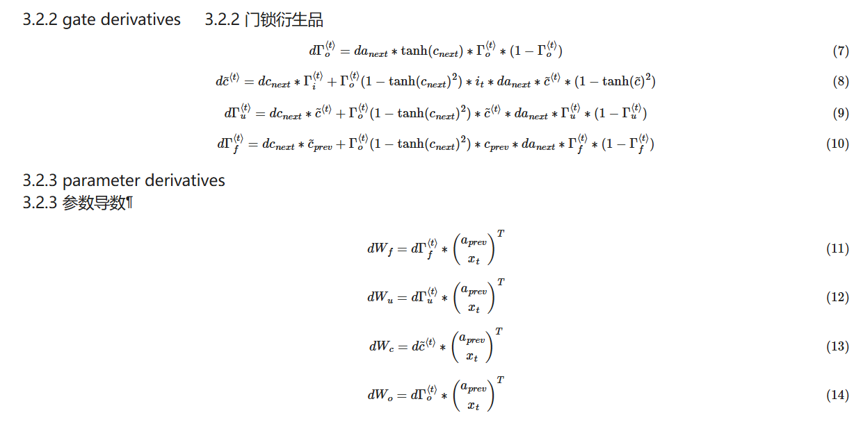
return a, y, c, caches4.2.2.6 向后传播
plain
def lstm_cell_backward(da_next, dc_next, cache):
    """
    Implement the backward pass for the LSTM-cell (single time-step).

    Arguments:
    da_next -- Gradients of next hidden state, of shape (n_a, m)
    dc_next -- Gradients of next cell state, of shape (n_a, m)
    cache -- cache storing information from the forward pass

    Returns:
    gradients -- python dictionary containing:
                        dxt -- Gradient of input data at time-step t, of shape (n_x, m)
                        da_prev -- Gradient w.r.t. the previous hidden state, numpy array of shape (n_a, m)
                        dc_prev -- Gradient w.r.t. the previous memory state, of shape (n_a, m, T_x)
                        dWf -- Gradient w.r.t. the weight matrix of the forget gate, numpy array of shape (n_a, n_a + n_x)
                        dWi -- Gradient w.r.t. the weight matrix of the input gate, numpy array of shape (n_a, n_a + n_x)
                        dWc -- Gradient w.r.t. the weight matrix of the memory gate, numpy array of shape (n_a, n_a + n_x)
                        dWo -- Gradient w.r.t. the weight matrix of the save gate, numpy array of shape (n_a, n_a + n_x)
                        dbf -- Gradient w.r.t. biases of the forget gate, of shape (n_a, 1)
                        dbi -- Gradient w.r.t. biases of the update gate, of shape (n_a, 1)
                        dbc -- Gradient w.r.t. biases of the memory gate, of shape (n_a, 1)
                        dbo -- Gradient w.r.t. biases of the save gate, of shape (n_a, 1)
    """

    # Retrieve information from "cache"
    (a_next, c_next, a_prev, c_prev, ft, it, cct, ot, xt, parameters) = cache

    ### START CODE HERE ###
    # Retrieve dimensions from xt's and a_next's shape (≈2 lines)
    n_x, m = xt.shape                                           # 取输入xt维度:n_x为输入特征数,m为batch大小
    n_a, m = a_next.shape                                       # 取隐藏状态a_next维度:n_a为隐藏单元数,m为batch大小

    # 先取出本时间步用到的参数矩阵(从parameters字典中读取)
    Wf = parameters["Wf"]                                       # 遗忘门权重矩阵 Wf,形状(n_a, n_a+n_x)
    Wi = parameters["Wi"]                                       # 输入/更新门权重矩阵 Wi,形状(n_a, n_a+n_x)
    Wc = parameters["Wc"]                                       # 候选记忆权重矩阵 Wc,形状(n_a, n_a+n_x)
    Wo = parameters["Wo"]                                       # 输出门权重矩阵 Wo,形状(n_a, n_a+n_x)

    # 拼接[a_prev; xt],用于计算参数梯度(与前向一致)
    concat = np.zeros((n_a + n_x, m))                            # 初始化拼接矩阵,形状(n_a+n_x, m)
    concat[:n_a, :] = a_prev                                     # 上半部分放a_prev
    concat[n_a:, :] = xt                                         # 下半部分放xt

    # Compute gates related derivatives, you can find their values can be found by looking carefully at equations (7) to (10) (≈4 lines)
    tanh_c_next = np.tanh(c_next)                                # 先算tanh(c_next),后面多处复用
    dot = da_next * tanh_c_next * ot * (1 - ot)                  # 输出门梯度:d(o_t) = da_next ⊙ tanh(c_next) ⊙ o_t(1-o_t)
    dc_next_total = dc_next + da_next * ot * (1 - tanh_c_next**2) # 合并流入c_next的梯度:原dc_next + 由a_next反传来的部分
    dc_prev = dc_next_total * ft                                 # 对上一记忆c_prev的梯度:dc_prev = dc_total ⊙ f_t(先算出来便于后面理解)

    # Code equations (7) to (10) (≈4 lines)
    dft = dc_next_total * c_prev * ft * (1 - ft)                 # 遗忘门梯度:d(f_t) = dc_total ⊙ c_prev ⊙ f_t(1-f_t)
    dit = dc_next_total * cct * it * (1 - it)                    # 输入门梯度:d(i_t) = dc_total ⊙ c~_t ⊙ i_t(1-i_t)
    dcct = dc_next_total * it * (1 - cct**2)                     # 候选记忆梯度:d(c~_t) = dc_total ⊙ i_t ⊙ (1-c~_t^2)
    # dc_prev 已在上面计算(等价于公式里的 dc_prev = dc_total ⊙ f_t)

    # Compute parameters related derivatives. Use equations (11)-(14) (≈8 lines)
    dWf = np.dot(dft, concat.T)                                  # Wf梯度:dWf = dft · concat^T,形状(n_a, n_a+n_x)
    dWi = np.dot(dit, concat.T)                                  # Wi梯度:dWi = dit · concat^T
    dWc = np.dot(dcct, concat.T)                                 # Wc梯度:dWc = dcct · concat^T
    dWo = np.dot(dot, concat.T)                                  # Wo梯度:dWo = dot · concat^T

    dbf = np.sum(dft, axis=1, keepdims=True)                     # bf梯度:对batch维求和,形状(n_a, 1)
    dbi = np.sum(dit, axis=1, keepdims=True)                     # bi梯度:对batch维求和
    dbc = np.sum(dcct, axis=1, keepdims=True)                    # bc梯度:对batch维求和
    dbo = np.sum(dot, axis=1, keepdims=True)                     # bo梯度:对batch维求和

    # Compute derivatives w.r.t previous hidden state, previous memory state and input. Use equations (15)-(17). (≈3 lines)
    dconcat = (np.dot(Wf.T, dft) + np.dot(Wi.T, dit) + np.dot(Wc.T, dcct) + np.dot(Wo.T, dot))  # 对拼接向量的梯度:各门反传梯度之和
    da_prev = dconcat[:n_a, :]                                    # 取dconcat上半部分作为对a_prev的梯度,形状(n_a, m)
    dxt = dconcat[n_a:, :]                                        # 取dconcat下半部分作为对xt的梯度,形状(n_x, m)
    ### END CODE HERE ###


    # Save gradients in dictionary
    gradients = {"dxt": dxt, "da_prev": da_prev, "dc_prev": dc_prev, "dWf": dWf,"dbf": dbf, "dWi": dWi,"dbi": dbi,
                "dWc": dWc,"dbc": dbc, "dWo": dWo,"dbo": dbo}

    return gradients
plain
def lstm_backward(da, caches):
"""
Implement the backward pass for the RNN with LSTM-cell (over a whole sequence).
Arguments:
da -- Gradients w.r.t the hidden states, numpy-array of shape (n_a, m, T_x)
dc -- Gradients w.r.t the memory states, numpy-array of shape (n_a, m, T_x)
caches -- cache storing information from the forward pass (lstm_forward)
Returns:
gradients -- python dictionary containing:
dx -- Gradient of inputs, of shape (n_x, m, T_x)
da0 -- Gradient w.r.t. the previous hidden state, numpy array of shape (n_a, m)
dWf -- Gradient w.r.t. the weight matrix of the forget gate, numpy array of shape (n_a, n_a + n_x)
dWi -- Gradient w.r.t. the weight matrix of the update gate, numpy array of shape (n_a, n_a + n_x)
dWc -- Gradient w.r.t. the weight matrix of the memory gate, numpy array of shape (n_a, n_a + n_x)
dWo -- Gradient w.r.t. the weight matrix of the save gate, numpy array of shape (n_a, n_a + n_x)
dbf -- Gradient w.r.t. biases of the forget gate, of shape (n_a, 1)
dbi -- Gradient w.r.t. biases of the update gate, of shape (n_a, 1)
dbc -- Gradient w.r.t. biases of the memory gate, of shape (n_a, 1)
dbo -- Gradient w.r.t. biases of the save gate, of shape (n_a, 1)
"""
# Retrieve values from the first cache (t=1) of caches.
(caches, x) = caches
(a1, c1, a0, c0, f1, i1, cc1, o1, x1, parameters) = caches[0]
### START CODE HERE ###
# Retrieve dimensions from da's and x1's shapes (≈2 lines)
n_a, m, T_x = da.shape # 从da获取维度:隐藏维度n_a、样本数m、时间步数T_x
n_x, m = x1.shape # 从x1获取输入维度n_x以及样本数m
# initialize the gradients with the right sizes (≈12 lines)
dx = np.zeros((n_x, m, T_x)) # 初始化对输入序列x的梯度dx,形状(n_x, m, T_x)
da0 = np.zeros((n_a, m)) # 初始化对初始隐藏状态a0的梯度(最后会赋值)
da_prev = np.zeros((n_a, m)) # 初始化来自未来时间步反传回来的隐藏梯度
dc_prev = np.zeros((n_a, m)) # 初始化来自未来时间步反传回来的记忆梯度(dc_next)
dWf = np.zeros((n_a, n_a + n_x)) # 初始化遗忘门权重梯度累加器
dWi = np.zeros((n_a, n_a + n_x)) # 初始化输入/更新门权重梯度累加器
dWc = np.zeros((n_a, n_a + n_x)) # 初始化候选记忆权重梯度累加器
dWo = np.zeros((n_a, n_a + n_x)) # 初始化输出门权重梯度累加器
dbf = np.zeros((n_a, 1)) # 初始化遗忘门偏置梯度累加器
dbi = np.zeros((n_a, 1)) # 初始化输入/更新门偏置梯度累加器
dbc = np.zeros((n_a, 1)) # 初始化候选记忆偏置梯度累加器
dbo = np.zeros((n_a, 1)) # 初始化输出门偏置梯度累加器
# loop back over the whole sequence
for t in reversed(range(T_x)): # 逆序遍历时间步:T_x-1 -> 0
# Compute all gradients using lstm_cell_backward
gradients_t = lstm_cell_backward(da[:, :, t] + da_prev, dc_prev, caches[t]) # 本步da_next=上游da_t+da_prev;dc_next用dc_prev(来自未来)
# Store or add the gradient to the parameters' previous step's gradient
dx[:, :, t] = gradients_t["dxt"] # 保存当前时间步对输入xt的梯度到dx的第t个切片
da_prev = gradients_t["da_prev"] # 更新da_prev,供前一个时间步(t-1)使用
dc_prev = gradients_t["dc_prev"] # 更新dc_prev,供前一个时间步(t-1)使用
dWf += gradients_t["dWf"] # 累加每个时间步的dWf
dWi += gradients_t["dWi"] # 累加每个时间步的dWi
dWc += gradients_t["dWc"] # 累加每个时间步的dWc
dWo += gradients_t["dWo"] # 累加每个时间步的dWo
dbf += gradients_t["dbf"] # 累加每个时间步的dbf
dbi += gradients_t["dbi"] # 累加每个时间步的dbi
dbc += gradients_t["dbc"] # 累加每个时间步的dbc
dbo += gradients_t["dbo"] # 累加每个时间步的dbo
# Set the first activation's gradient to the backpropagated gradient da_prev.
da0 = da_prev # 反传完成后,da_prev就是对初始隐藏状态a0的梯度
### END CODE HERE ###
# Store the gradients in a python dictionary
gradients = {"dx": dx, "da0": da0, "dWf": dWf,"dbf": dbf, "dWi": dWi,"dbi": dbi,
"dWc": dWc,"dbc": dbc, "dWo": dWo,"dbo": dbo}
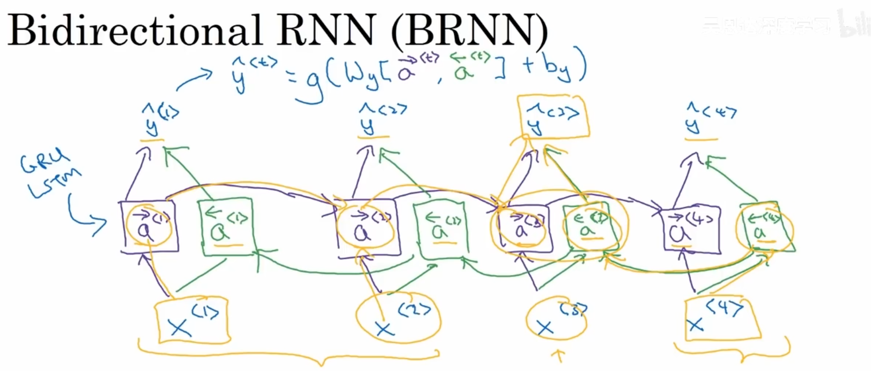
return gradients五、双向递归神经网络(BRNN)
将向前传播修改为2个部分,一部分是从左到右,另一部分是从右到左。每一层的预测值综合了之前和之后的信息。
六、深度RNNs
深度RNNs意味着一层神经网络还有很多层激活层:
