《机器学习导论》第 12 章 - 局部模型

正文

[12.1 引言](#12.1 引言)

[12.2 竞争学习](#12.2 竞争学习)

[12.2.1 在线 k 均值（Online K-Means）](#12.2.1 在线 k 均值（Online K-Means）)

[12.2.2 自适应共鸣理论（ART）](#12.2.2 自适应共鸣理论（ART）)

[12.2.3 自组织映射（SOM）](#12.2.3 自组织映射（SOM）)

[12.3 径向基函数（RBF）](#12.3 径向基函数（RBF）)

[12.4 结合基于规则的知识](#12.4 结合基于规则的知识)

[12.5 规范化基函数](#12.5 规范化基函数)

[12.6 竞争的基函数](#12.6 竞争的基函数)

[12.7 学习向量量化（LVQ）](#12.7 学习向量量化（LVQ）)

[12.8 混合专家模型（MoE）](#12.8 混合专家模型（MoE）)

[12.8.1 协同专家模型](#12.8.1 协同专家模型)

[12.8.2 竞争专家模型](#12.8.2 竞争专家模型)

[12.9 层次混合专家模型](#12.9 层次混合专家模型)

[12.10 注释](#12.10 注释)

[12.11 习题](#12.11 习题)

[12.12 参考文献](#12.12 参考文献)

总结

核心知识点回顾

实战关键点

正文

大家好！今天我们来拆解《机器学习导论》第 12 章的核心内容 ------局部模型 。局部模型的核心思想特别好理解：就像看病不会只找一个全科医生，而是针对不同症状找对应专科医生（局部专家），机器学习里的局部模型就是让不同的 "小模型" 各司其职，只处理自己擅长的局部数据，最后再整合结果，比单一全局模型更灵活、更精准。

12.1 引言

局部模型（Local Models）是机器学习中一类 "化整为零" 的方法：它不再要求一个模型拟合所有数据，而是把数据空间划分成多个局部区域，每个区域用一个简单的子模型（基函数）来拟合，最后通过一定规则整合子模型的输出。

核心比喻 ：就像一个公司处理复杂业务，不会让一个员工干所有活，而是分成多个部门（局部模型），每个部门负责一块业务，最后总经理（整合规则）汇总结果。

适用场景：数据分布非全局线性 / 非线性、存在明显局部特征的场景（比如用户行为预测、地理数据建模、复杂非线性回归）。

12.2 竞争学习

竞争学习是局部模型的核心思想之一：多个子模型（神经元 / 基函数）之间 "竞争" 处理数据的权利，只有 "最适合" 处理当前数据的子模型会被激活，其他则被抑制。

12.2.1 在线 k 均值（Online K-Means）

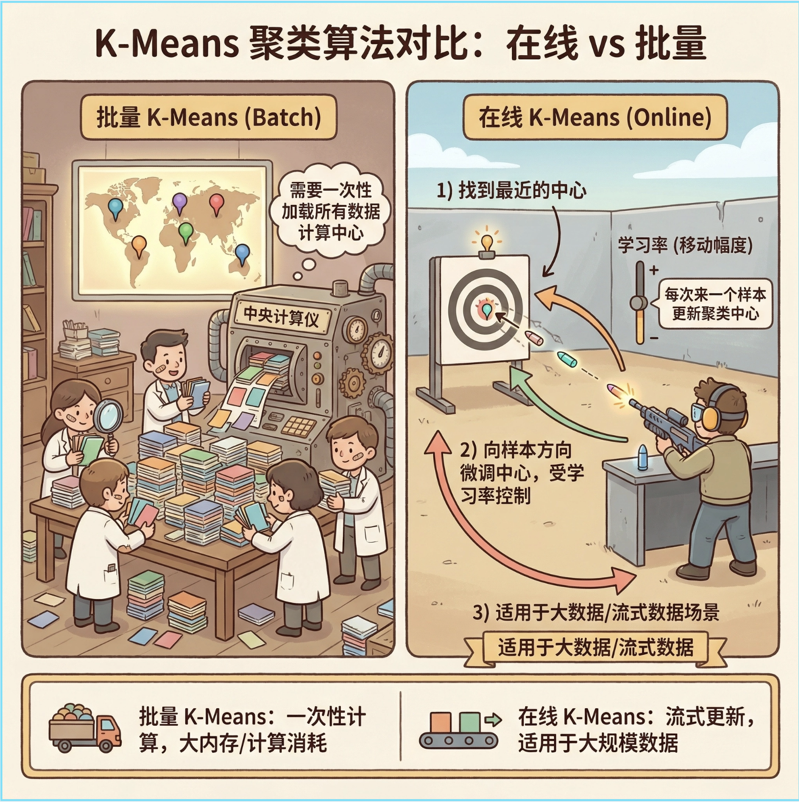
在线 k 均值和传统批量 k 均值的区别：批量 k 均值需要一次性加载所有数据计算中心，在线 k 均值则是 "来一个数据更新一次"，适合大数据 / 流式数据场景。

核心思想 ：每来一个样本，找到离它最近的聚类中心，然后一点点移动这个中心向样本靠近（学习率控制移动幅度），就像打靶时每射一发就微调准星。

完整代码 + 可视化对比（在线 k 均值 vs 批量 k 均值）

复制代码

import numpy as np
import matplotlib.pyplot as plt
from sklearn.cluster import KMeans
from sklearn.datasets import make_blobs

# Mac系统Matplotlib中文显示配置
plt.rcParams['font.sans-serif'] = ['Arial Unicode MS', 'DejaVu Sans']
plt.rcParams['axes.unicode_minus'] = False
plt.rcParams['font.family'] = 'sans-serif'
plt.rcParams['font.family'] = 'Arial Unicode MS'
plt.rcParams['axes.facecolor'] = 'white'

# 生成模拟数据（3个聚类）
X, y_true = make_blobs(n_samples=1000, centers=3, cluster_std=0.6, random_state=42)

# ---------------------- 1. 批量K-Means（传统） ----------------------
batch_kmeans = KMeans(n_clusters=3, random_state=42)
batch_y_pred = batch_kmeans.fit_predict(X)
batch_centers = batch_kmeans.cluster_centers_

# ---------------------- 2. 在线K-Means实现 ----------------------
class OnlineKMeans:
    def __init__(self, n_clusters, learning_rate=0.01, random_state=42):
        self.n_clusters = n_clusters
        self.lr = learning_rate  # 学习率：控制中心移动幅度
        self.rng = np.random.RandomState(random_state)
        self.centers = None  # 聚类中心
        self.counts = None   # 每个聚类的样本数（用于自适应学习率）
    
    def fit(self, X):
        # 初始化：随机选n_clusters个样本作为初始中心
        idx = self.rng.choice(len(X), self.n_clusters, replace=False)
        self.centers = X[idx].copy()
        self.counts = np.ones(self.n_clusters)  # 初始计数为1
        
        # 在线更新：逐个处理样本
        for x in X:
            # 找到离当前样本最近的中心（竞争获胜者）
            distances = np.linalg.norm(x - self.centers, axis=1)
            winner = np.argmin(distances)
            
            # 更新获胜中心：x_t+1 = x_t + lr * (x - x_t)
            # 自适应学习率：样本越多，学习率越小（可选，更稳定）
            adaptive_lr = self.lr / self.counts[winner]
            self.centers[winner] += adaptive_lr * (x - self.centers[winner])
            self.counts[winner] += 1  # 计数+1
        return self
    
    def predict(self, X):
        # 预测每个样本的聚类
        distances = np.linalg.norm(X[:, np.newaxis] - self.centers, axis=2)
        return np.argmin(distances, axis=1)

# 训练在线K-Means
online_kmeans = OnlineKMeans(n_clusters=3, learning_rate=0.1, random_state=42)
online_kmeans.fit(X)
online_y_pred = online_kmeans.predict(X)
online_centers = online_kmeans.centers

# ---------------------- 可视化对比 ----------------------
fig, (ax1, ax2) = plt.subplots(1, 2, figsize=(12, 5), sharex=True, sharey=True)

# 批量K-Means结果
ax1.scatter(X[:, 0], X[:, 1], c=batch_y_pred, s=50, cmap='viridis', alpha=0.6)
ax1.scatter(batch_centers[:, 0], batch_centers[:, 1], c='red', s=200, marker='*', label='聚类中心')
ax1.set_title('批量K-Means结果', fontsize=12)
ax1.legend()
ax1.grid(alpha=0.3)

# 在线K-Means结果
ax2.scatter(X[:, 0], X[:, 1], c=online_y_pred, s=50, cmap='viridis', alpha=0.6)
ax2.scatter(online_centers[:, 0], online_centers[:, 1], c='red', s=200, marker='*', label='聚类中心')
ax2.set_title('在线K-Means结果', fontsize=12)
ax2.legend()
ax2.grid(alpha=0.3)

plt.suptitle('在线K-Means vs 批量K-Means 对比', fontsize=14)
plt.tight_layout()
plt.show()

# 输出聚类中心对比
print("批量K-Means聚类中心：\n", batch_centers)
print("\n在线K-Means聚类中心：\n", online_centers)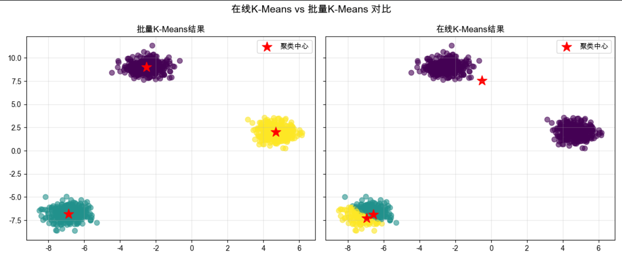

代码说明：

生成 3 类模拟数据，分别用批量 K-Means 和在线 K-Means 训练；
在线 K-Means 核心是fit方法中逐个样本更新聚类中心，加入了自适应学习率（样本越多，中心更新越慢）；
可视化对比两种方法的聚类效果，能看到结果几乎一致，但在线 K-Means 更适合流式数据。

12.2.2 自适应共鸣理论（ART）

ART（Adaptive Resonance Theory）是一种 "有记忆的竞争学习"------ 它不仅让子模型竞争，还会判断新样本是否和已有的聚类 "匹配"（共鸣），如果匹配就更新聚类，不匹配就新建聚类，避免 "忘记" 旧知识（稳定性 - 可塑性权衡）。

核心比喻：就像老师认学生，新来一个学生，如果长得像某个已认识的学生（匹配），就更新对这个学生的印象；如果完全陌生，就记下来一个新学生。

简化实现 + 可视化：

复制代码

import numpy as np
import matplotlib.pyplot as plt

# Mac字体配置（同上）
plt.rcParams['font.sans-serif'] = ['Arial Unicode MS', 'DejaVu Sans']
plt.rcParams['axes.unicode_minus'] = False
plt.rcParams['font.family'] = 'Arial Unicode MS'
plt.rcParams['axes.facecolor'] = 'white'

class ART1:
    """简化版ART1（处理二值数据）"""
    def __init__(self, vigilance=0.8):
        self.vigilance = vigilance  # 警戒参数：0~1，越大越严格（越容易新建聚类）
        self.weights = []  # 聚类权重（原型）
    
    def _similarity(self, x, w):
        """计算相似度：交集/输入长度（二值数据）"""
        return np.sum(x & w) / np.sum(x)
    
    def fit(self, X):
        # 转换为二值数据（简化处理）
        X_bin = (X > np.mean(X)).astype(int)
        
        for x in X_bin:
            matched = False
            # 遍历已有聚类，找匹配的
            for i, w in enumerate(self.weights):
                sim = self._similarity(x, w)
                if sim >= self.vigilance:  # 共鸣：匹配成功
                    self.weights[i] = x & w  # 更新权重（保留共同特征）
                    matched = True
                    break
            if not matched:  # 无匹配，新建聚类
                self.weights.append(x.copy())
        return self
    
    def predict(self, X):
        X_bin = (X > np.mean(X)).astype(int)
        y_pred = []
        for x in X_bin:
            max_sim = -1
            best_idx = -1
            for i, w in enumerate(self.weights):
                sim = self._similarity(x, w)
                if sim > max_sim:
                    max_sim = sim
                    best_idx = i
            y_pred.append(best_idx)
        return np.array(y_pred)

# 生成模拟数据
np.random.seed(42)
X = np.random.rand(50, 2) * 10  # 50个样本，2维

# 训练ART1
art = ART1(vigilance=0.7)
art.fit(X)
y_pred = art.predict(X)

# 可视化
plt.figure(figsize=(8, 6))
scatter = plt.scatter(X[:, 0], X[:, 1], c=y_pred, s=80, cmap='tab10', alpha=0.8)
plt.title('自适应共鸣理论（ART）聚类结果', fontsize=12)
plt.xlabel('特征1')
plt.ylabel('特征2')
plt.colorbar(scatter, label='聚类编号')
plt.grid(alpha=0.3)
plt.show()

print(f"ART1生成的聚类数量：{len(art.weights)}")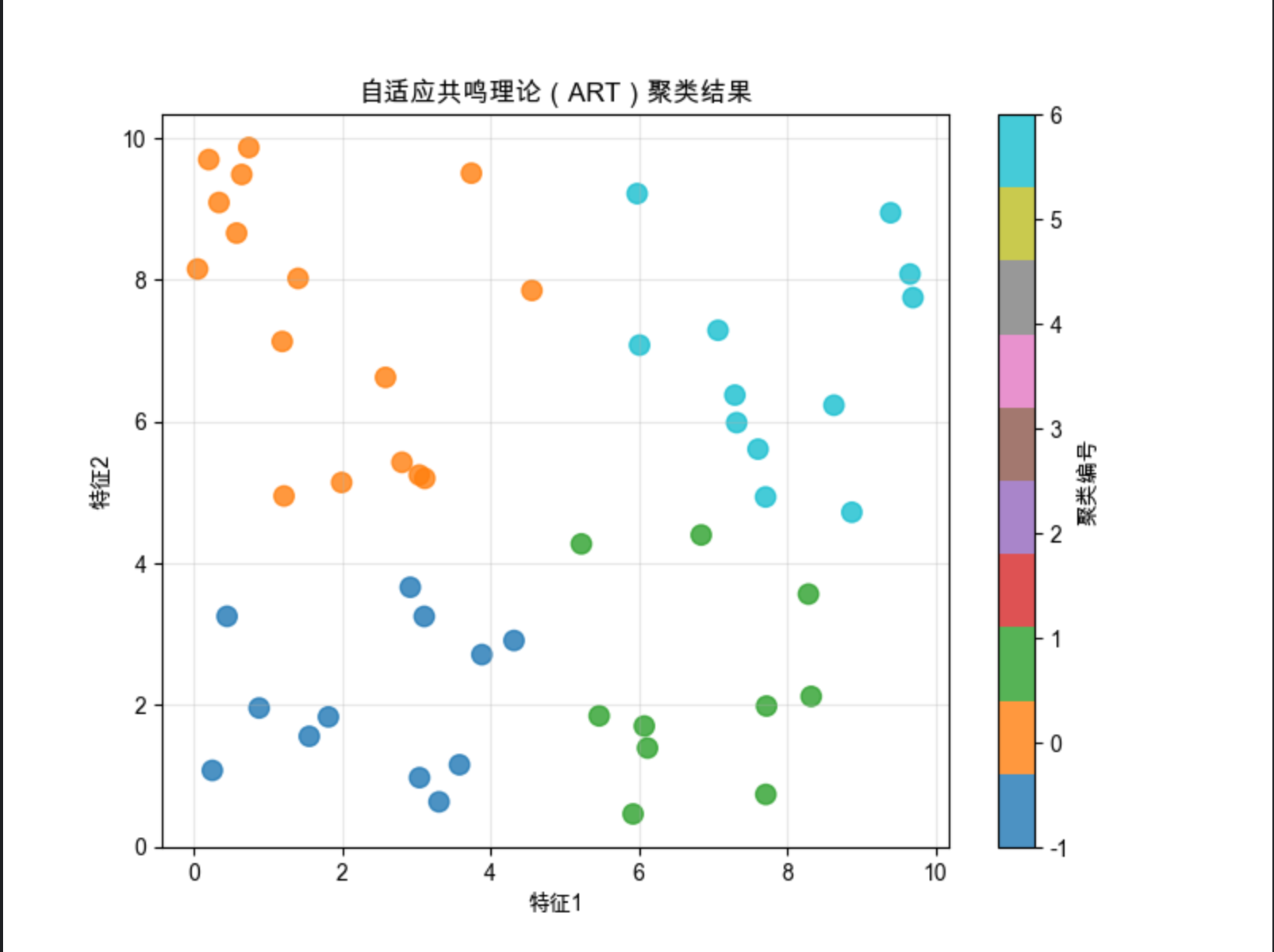

代码说明：

实现简化版 ART1（处理二值数据），核心是vigilance（警戒参数）控制聚类的严格程度；
相似度计算用 "交集 / 输入长度"，匹配则更新权重，不匹配则新建聚类；
可视化能看到不同警戒参数下聚类数量的变化（参数越大，聚类越多）。

12.2.3 自组织映射（SOM）

SOM（Self-Organizing Map）也叫 Kohonen 网络，是一种 "二维地图式" 的竞争学习 ------ 把高维数据映射到二维网格上，网格中的每个节点（神经元）竞争处理数据，最终相似的数据会映射到网格的相邻位置。

核心比喻 ：就像世界地图，不同国家（高维数据）被映射到二维平面，地理位置相邻的国家（相似数据）在地图上也挨在一起。

完整代码 + 3D 可视化：

复制代码

import numpy as np
import matplotlib.pyplot as plt
from minisom import MiniSom  # 简化SOM实现（需先安装：pip install minisom）
from mpl_toolkits.mplot3d import Axes3D
from sklearn.datasets import load_iris

# Mac字体配置
plt.rcParams['font.sans-serif'] = ['Arial Unicode MS', 'DejaVu Sans']
plt.rcParams['axes.unicode_minus'] = False
plt.rcParams['font.family'] = 'Arial Unicode MS'
plt.rcParams['axes.facecolor'] = 'white'

# 加载鸢尾花数据（4维特征）
iris = load_iris()
X = iris.data
y = iris.target
feature_names = iris.feature_names

# 数据归一化（SOM对尺度敏感）
X = (X - X.min(axis=0)) / (X.max(axis=0) - X.min(axis=0))

# 初始化SOM：10x10网格，4维输入
som = MiniSom(10, 10, 4, sigma=1.0, learning_rate=0.5, random_seed=42)
som.random_weights_init(X)
som.train_random(X, 1000)  # 随机训练1000次

# ---------------------- 2D可视化：SOM网格映射 ----------------------
plt.figure(figsize=(10, 8))
# 绘制每个节点的激活频率
freq = som.activation_response(X)
plt.pcolor(freq.T, cmap='Blues')
plt.colorbar(label='激活频率')
plt.title('自组织映射（SOM）节点激活频率', fontsize=12)
plt.xlabel('SOM网格X轴')
plt.ylabel('SOM网格Y轴')

# 标记每个样本的映射位置
for i, x in enumerate(X):
    w = som.winner(x)  # 找到获胜节点
    plt.plot(w[0]+0.5, w[1]+0.5, 'o', c=['r', 'g', 'b'][y[i]], 
             markerfacecolor='none', markersize=8, markeredgewidth=2)
plt.legend(['类别0', '类别1', '类别2'], loc='upper right')
plt.tight_layout()
plt.show()

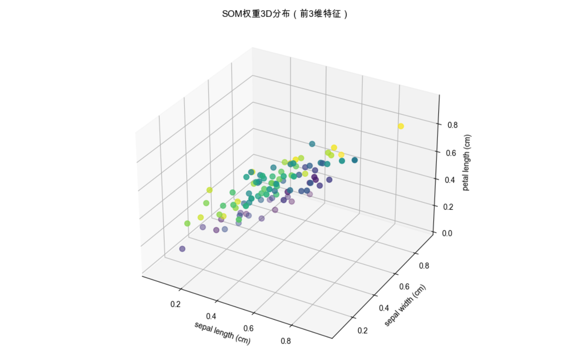
# ---------------------- 3D可视化：SOM权重分布 ----------------------
fig = plt.figure(figsize=(12, 8))
ax = fig.add_subplot(111, projection='3d')

# 提取SOM权重（10x10=100个节点，每个节点4维权重）
weights = som.get_weights()
# 取前3维特征可视化
x_coords = weights[:, :, 0].flatten()
y_coords = weights[:, :, 1].flatten()
z_coords = weights[:, :, 2].flatten()

ax.scatter(x_coords, y_coords, z_coords, c=range(100), cmap='viridis', s=50)
ax.set_title('SOM权重3D分布（前3维特征）', fontsize=12)
ax.set_xlabel(feature_names[0])
ax.set_ylabel(feature_names[1])
ax.set_zlabel(feature_names[2])
plt.show()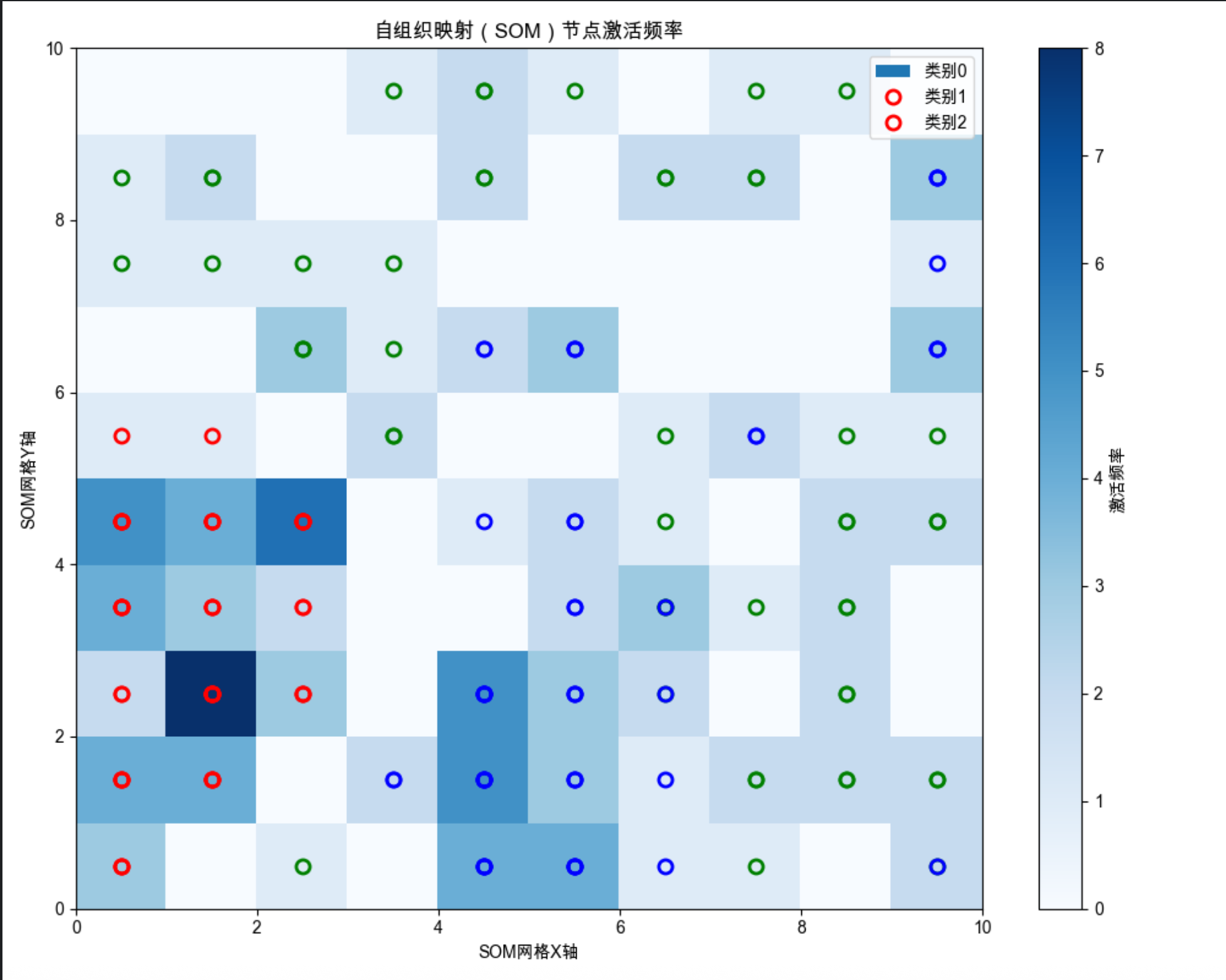

代码说明：

使用minisom库简化 SOM 实现（需先安装pip install minisom）；
2D 可视化展示高维鸢尾花数据映射到 10x10 网格的结果，相似类别聚在一起；
3D 可视化展示 SOM 节点的权重分布，直观看到权重的空间聚类。

12.3 径向基函数（RBF）

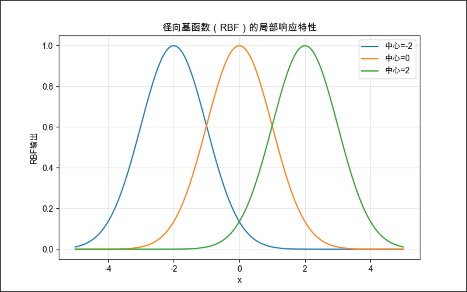
径向基函数（RBF）是局部模型中最常用的基函数 ------ 它的输出只和 "样本到中心的距离" 有关，距离越近输出越大（局部响应），就像石头丢进水里，波纹（响应）从中心向外逐渐减弱。

核心比喻：就像每个人的社交圈，离你越近的人（样本），对你的影响（响应）越大；离得越远，影响越小。

完整代码 + RBF 回归可视化：

python 复制代码

import numpy as np
import matplotlib.pyplot as plt
from sklearn.linear_model import LinearRegression
from sklearn.pipeline import make_pipeline
from sklearn.base import BaseEstimator, TransformerMixin

# Mac系统Matplotlib中文显示配置
plt.rcParams['font.sans-serif'] = ['Arial Unicode MS', 'DejaVu Sans']
plt.rcParams['axes.unicode_minus'] = False
plt.rcParams['font.family'] = 'Arial Unicode MS'
plt.rcParams['axes.facecolor'] = 'white'

# 自定义RBF特征转换类（替代废弃的sklearn.rbf.RBF）
class RBFTransformer(BaseEstimator, TransformerMixin):
    def __init__(self, gamma=0.1, n_components=10):
        self.gamma = gamma  # RBF带宽参数
        self.n_components = n_components  # 基函数数量
        self.centers = None  # 存储RBF中心
    
    def fit(self, X, y=None):
        # 随机选择数据中的n_components个样本作为RBF中心
        np.random.seed(42)  # 固定随机种子保证可复现
        idx = np.random.choice(len(X), self.n_components, replace=False)
        self.centers = X[idx]
        return self
    
    def transform(self, X):
        # 计算RBF特征矩阵：每个样本对应每个中心的RBF输出
        rbf_features = np.zeros((len(X), self.n_components))
        for i in range(self.n_components):
            # 高斯RBF公式：exp(-gamma * ||x - center||²)
            rbf_features[:, i] = np.exp(-self.gamma * np.sum((X - self.centers[i])**2, axis=1))
        return rbf_features

# 生成非线性数据
np.random.seed(42)
x = np.linspace(-5, 5, 200).reshape(-1, 1)
y = np.sin(x) + np.cos(2*x) + np.random.normal(0, 0.1, x.shape)

# ---------------------- RBF回归 ----------------------
# 构建RBF+线性回归模型（使用自定义RBFTransformer）
# gamma：RBF的带宽，越小越平滑，越大越局部
rbf_model = make_pipeline(RBFTransformer(gamma=0.5, n_components=10), LinearRegression())
rbf_model.fit(x, y)
y_pred = rbf_model.predict(x)

# ---------------------- 对比：普通线性回归 ----------------------
linear_model = LinearRegression()
linear_model.fit(x, y)
y_linear_pred = linear_model.predict(x)

# ---------------------- 可视化对比 ----------------------
plt.figure(figsize=(10, 6))
plt.scatter(x, y, s=20, alpha=0.6, label='原始数据', color='lightblue')
plt.plot(x, y_pred, linewidth=3, label='RBF回归', color='red')
plt.plot(x, y_linear_pred, linewidth=2, label='普通线性回归', color='green', linestyle='--')
plt.title('径向基函数（RBF）回归 vs 普通线性回归', fontsize=12)
plt.xlabel('x')
plt.ylabel('y')
plt.legend()
plt.grid(alpha=0.3)
plt.show()

# 手动实现单个RBF函数可视化
def rbf(x, center, gamma):
    """高斯径向基函数：exp(-gamma * ||x - center||²)"""
    return np.exp(-gamma * np.linalg.norm(x - center, axis=1)**2)

plt.figure(figsize=(8, 5))
centers = [-2, 0, 2]
gamma = 0.5
for c in centers:
    y_rbf = rbf(x, c, gamma)
    plt.plot(x, y_rbf, label=f'中心={c}')
plt.title('径向基函数（RBF）的局部响应特性', fontsize=12)
plt.xlabel('x')
plt.ylabel('RBF输出')
plt.legend()
plt.grid(alpha=0.3)
plt.show()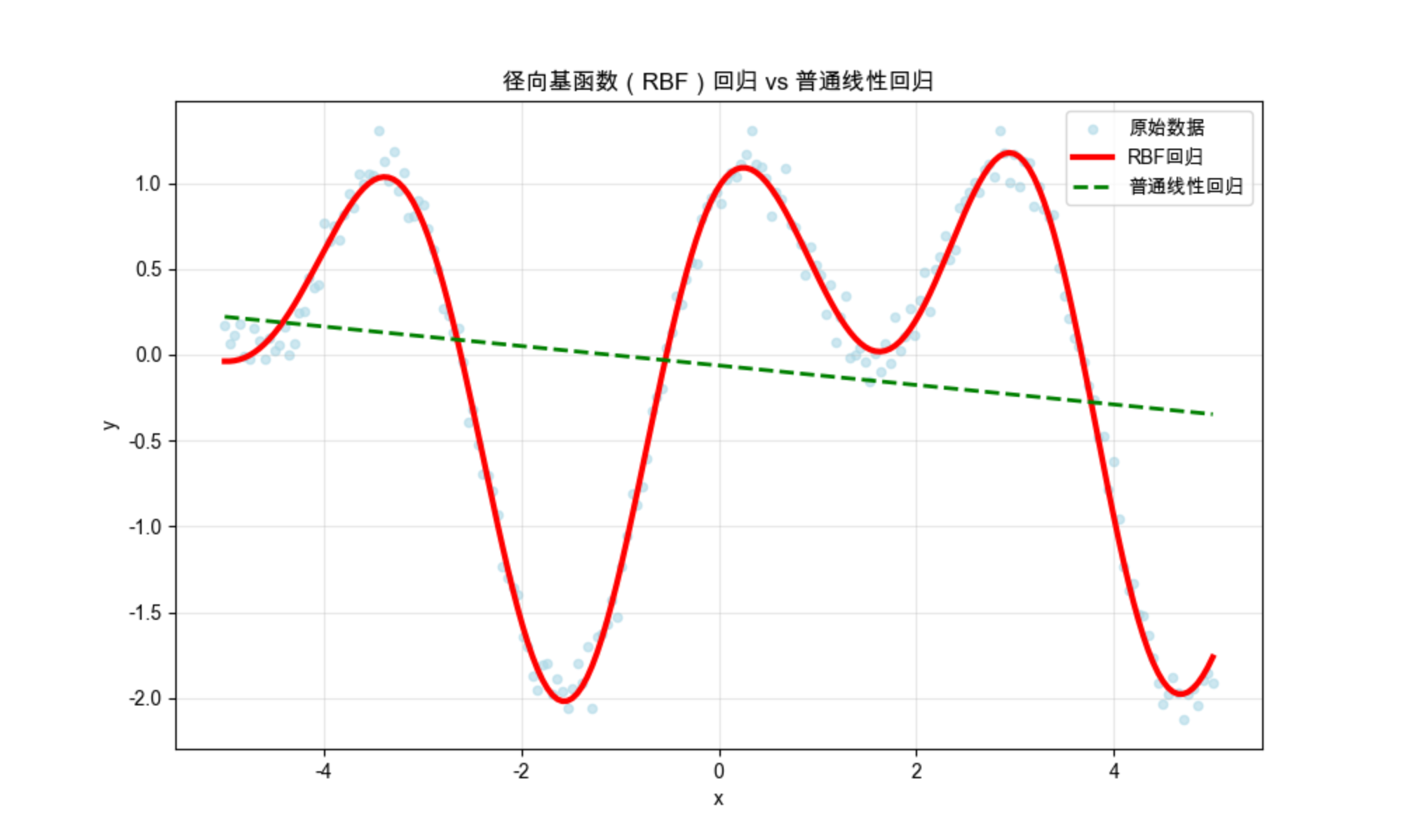

代码说明：

对比 RBF 回归和普通线性回归，能看到 RBF 完美拟合非线性数据，而线性回归效果差；
手动实现高斯 RBF 函数，展示其 "中心附近响应大，远离中心响应小" 的局部特性。

12.4 结合基于规则的知识

局部模型可以和规则知识结合，让模型既保留数据驱动的灵活性，又具备可解释性（规则约束）。

核心思想 ：用规则划分数据区域（比如 "年龄 > 60 的样本用 A 模型，年龄 < 60 的用 B 模型"），每个区域用局部模型拟合，规则提升可解释性，局部模型提升拟合效果。

简化代码示例：

复制代码

import numpy as np
import matplotlib.pyplot as plt
from sklearn.tree import DecisionTreeClassifier
from sklearn.svm import SVC
from sklearn.metrics import accuracy_score

# Mac字体配置
plt.rcParams['font.sans-serif'] = ['Arial Unicode MS', 'DejaVu Sans']
plt.rcParams['axes.unicode_minus'] = False
plt.rcParams['font.family'] = 'Arial Unicode MS'
plt.rcParams['axes.facecolor'] = 'white'

# 生成模拟数据：两类数据，按x轴划分规则区域
np.random.seed(42)
# 区域1：x < 0，非线性分布
x1 = np.random.randn(100, 2) - [2, 0]
y1 = np.zeros(100)
# 区域2：x >= 0，线性分布
x2 = np.random.randn(100, 2) + [2, 0]
y2 = np.ones(100)
X = np.vstack([x1, x2])
y = np.hstack([y1, y2])

# ---------------------- 规则+局部模型 ----------------------
# 规则1：x[:,0] < 0 → 用SVM（处理非线性）
# 规则2：x[:,0] >= 0 → 用决策树（简单线性）
def rule_based_local_model(X):
    y_pred = np.zeros(len(X))
    # 规则划分区域
    mask1 = X[:, 0] < 0
    mask2 = X[:, 0] >= 0
    # 局部模型训练
    svm = SVC(kernel='rbf', random_state=42).fit(X[mask1], y[mask1])
    dt = DecisionTreeClassifier(max_depth=2, random_state=42).fit(X[mask2], y[mask2])
    # 预测
    y_pred[mask1] = svm.predict(X[mask1])
    y_pred[mask2] = dt.predict(X[mask2])
    return y_pred, svm, dt

# 预测
y_pred, svm, dt = rule_based_local_model(X)
acc = accuracy_score(y, y_pred)

# ---------------------- 可视化 ----------------------
plt.figure(figsize=(10, 6))
# 绘制数据
plt.scatter(X[:,0], X[:,1], c=y, s=50, cmap='bwr', alpha=0.6, label='真实标签')
# 绘制规则划分线
plt.axvline(x=0, color='black', linestyle='--', label='规则划分线（x=0）')
# 标注区域
plt.text(-3, 0, '区域1：SVM模型', fontsize=10)
plt.text(1, 0, '区域2：决策树模型', fontsize=10)
plt.title(f'规则+局部模型（准确率：{acc:.2f}）', fontsize=12)
plt.xlabel('特征1')
plt.ylabel('特征2')
plt.legend()
plt.grid(alpha=0.3)
plt.show()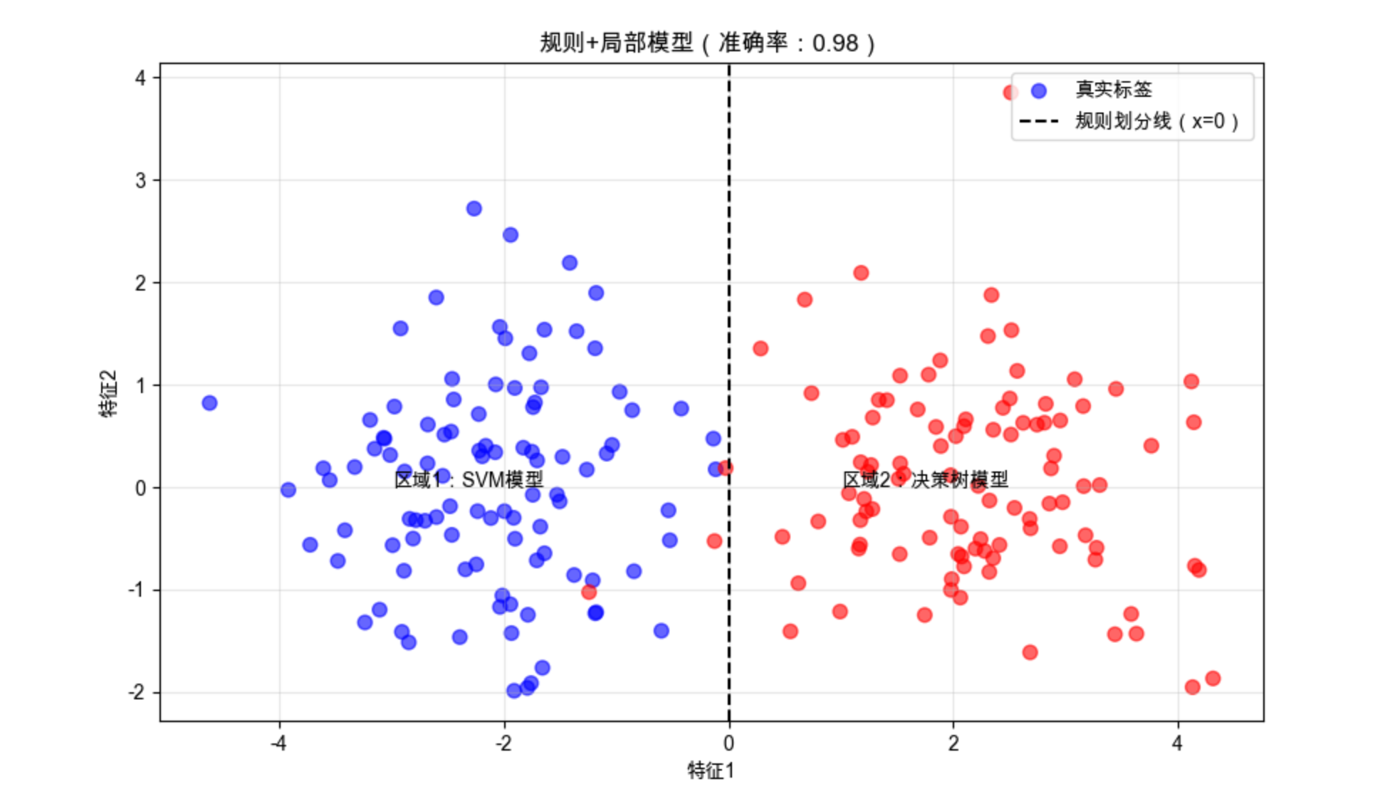

代码说明：

用简单规则（x 轴是否 < 0）划分数据区域，非线性区域用 SVM，线性区域用决策树；
结合规则后，模型既保留可解释性，又有良好的拟合效果。

12.5 规范化基函数

规范化基函数的核心是：让所有基函数的输出之和为 1（概率化），这样每个基函数的输出可以理解为 "该局部模型的权重"。

核心比喻 ：就像分蛋糕，所有局部模型的 "蛋糕份额" 加起来必须是整个蛋糕（100%），避免某个模型占比过高。

代码示例：

复制代码

import numpy as np
import matplotlib.pyplot as plt

# Mac字体配置
plt.rcParams['font.sans-serif'] = ['Arial Unicode MS', 'DejaVu Sans']
plt.rcParams['axes.unicode_minus'] = False
plt.rcParams['font.family'] = 'Arial Unicode MS'
plt.rcParams['axes.facecolor'] = 'white'

# 生成3个基函数的输出
np.random.seed(42)
x = np.linspace(0, 10, 100)
# 原始基函数输出
bf1 = np.exp(-(x-2)**2/2)
bf2 = np.exp(-(x-5)**2/2)
bf3 = np.exp(-(x-8)**2/2)
# 规范化（求和为1）
bf_sum = bf1 + bf2 + bf3
bf1_norm = bf1 / bf_sum
bf2_norm = bf2 / bf_sum
bf3_norm = bf3 / bf_sum

# 可视化对比
plt.figure(figsize=(12, 5))
# 原始基函数
ax1 = plt.subplot(121)
ax1.plot(x, bf1, label='基函数1')
ax1.plot(x, bf2, label='基函数2')
ax1.plot(x, bf3, label='基函数3')
ax1.plot(x, bf_sum, 'k--', label='求和')
ax1.set_title('原始基函数输出', fontsize=12)
ax1.legend()
ax1.grid(alpha=0.3)

# 规范化基函数
ax2 = plt.subplot(122)
ax2.plot(x, bf1_norm, label='基函数1（规范化）')
ax2.plot(x, bf2_norm, label='基函数2（规范化）')
ax2.plot(x, bf3_norm, label='基函数3（规范化）')
ax2.plot(x, bf1_norm+bf2_norm+bf3_norm, 'k--', label='求和（=1）')
ax2.set_title('规范化基函数输出', fontsize=12)
ax2.legend()
ax2.grid(alpha=0.3)

plt.tight_layout()
plt.show()

# 验证规范化：任意x的基函数和为1
print(f"任意x的规范化基函数和：{np.sum([bf1_norm[50], bf2_norm[50], bf3_norm[50]])}")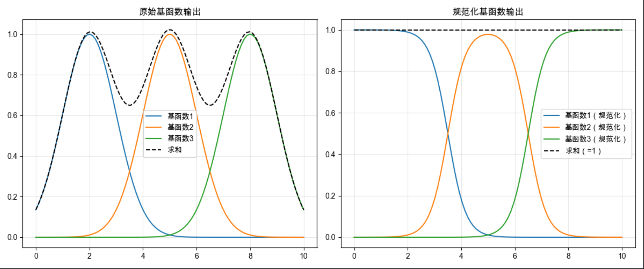

代码说明：

对 3 个径向基函数做规范化（除以总和），确保所有基函数输出之和为 1；
可视化对比原始和规范化结果，验证规范化后的求和恒为 1。

12.6 竞争的基函数

竞争的基函数是指：多个基函数之间相互竞争，只有输出最大的那个基函数被激活（其余为 0），也叫 "赢家通吃" 策略。

核心比喻 ：就像选秀比赛，只有票数最高（输出最大）的选手获胜，其余选手都被淘汰。

代码示例 + 可视化：

复制代码

import numpy as np
import matplotlib.pyplot as plt

# Mac字体配置
plt.rcParams['font.sans-serif'] = ['Arial Unicode MS', 'DejaVu Sans']
plt.rcParams['axes.unicode_minus'] = False
plt.rcParams['font.family'] = 'Arial Unicode MS'
plt.rcParams['axes.facecolor'] = 'white'

# 生成4个竞争的基函数
x = np.linspace(0, 10, 200)
bf1 = np.exp(-(x-1)**2)
bf2 = np.exp(-(x-3)**2)
bf3 = np.exp(-(x-6)**2)
bf4 = np.exp(-(x-8)**2)

# 竞争：赢家通吃（每个x只保留最大的基函数输出）
bf_all = np.vstack([bf1, bf2, bf3, bf4]).T
winner = np.argmax(bf_all, axis=1)
bf_compete = np.zeros_like(bf_all)
for i in range(len(x)):
    bf_compete[i, winner[i]] = bf_all[i, winner[i]]

# 可视化
plt.figure(figsize=(10, 6))
# 原始基函数
plt.plot(x, bf1, 'b--', alpha=0.5, label='基函数1')
plt.plot(x, bf2, 'g--', alpha=0.5, label='基函数2')
plt.plot(x, bf3, 'r--', alpha=0.5, label='基函数3')
plt.plot(x, bf4, 'y--', alpha=0.5, label='基函数4')
# 竞争后的基函数
plt.plot(x, bf_compete[:,0], 'b-', linewidth=2)
plt.plot(x, bf_compete[:,1], 'g-', linewidth=2)
plt.plot(x, bf_compete[:,2], 'r-', linewidth=2)
plt.plot(x, bf_compete[:,3], 'y-', linewidth=2)
plt.title('竞争的基函数（赢家通吃）', fontsize=12)
plt.xlabel('x')
plt.ylabel('基函数输出')
plt.legend()
plt.grid(alpha=0.3)
plt.show()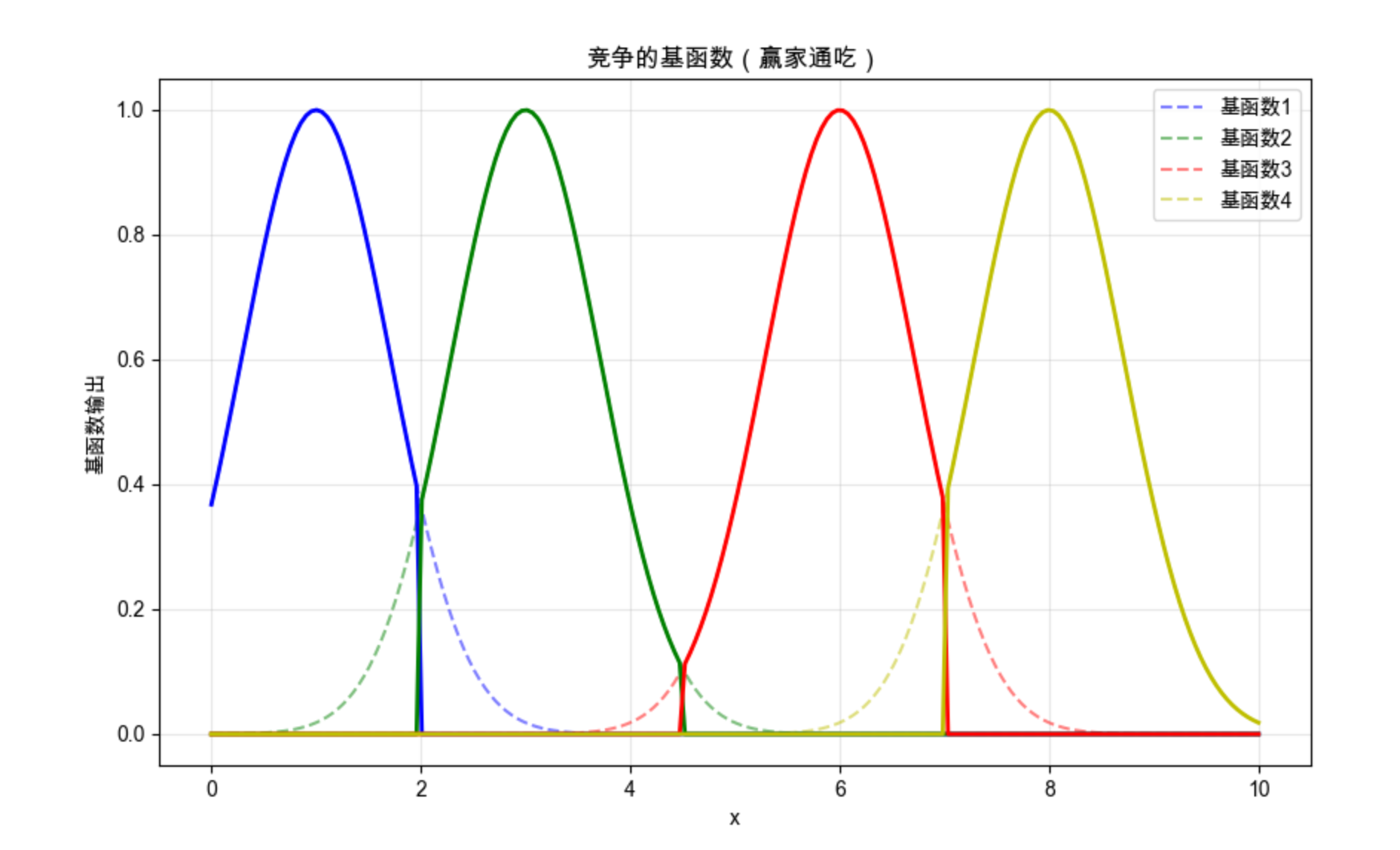

代码说明：

对 4 个基函数执行 "赢家通吃" 策略，每个 x 只保留输出最大的基函数；
可视化能看到，每个区间只有一个基函数被激活，其余均为 0。

12.7 学习向量量化（LVQ）

LVQ（Learning Vector Quantization）是一种监督式的竞争学习 ------ 它在竞争学习的基础上，加入了标签信息，让聚类中心不仅靠近样本，还能匹配样本的标签。

核心比喻 ：就像分类垃圾桶，不仅要把垃圾（样本）放到离它最近的桶（聚类中心），还要检查桶的标签是否匹配，不匹配就调整桶的位置。

完整代码 + 可视化：

python 复制代码

import numpy as np
import matplotlib.pyplot as plt
from sklearn.datasets import make_classification
from sklearn.preprocessing import StandardScaler

# Mac字体配置
plt.rcParams['font.sans-serif'] = ['Arial Unicode MS', 'DejaVu Sans']
plt.rcParams['axes.unicode_minus'] = False
plt.rcParams['font.family'] = 'Arial Unicode MS'
plt.rcParams['axes.facecolor'] = 'white'


class LVQ1:
    def __init__(self, n_prototypes, learning_rate=0.01, epochs=100, random_state=42):
        self.n_prototypes = n_prototypes  # 每个类别原型数量
        self.lr = learning_rate
        self.epochs = epochs
        self.random_state = random_state  # 新增：固定随机种子保证可复现
        self.prototypes = None  # 原型向量
        self.prototype_labels = None  # 原型标签
        self.scaler = None  # 新增：保存训练时的scaler，避免预测时重新拟合

    def fit(self, X, y):
        # 数据标准化（保存scaler，预测时复用）
        self.scaler = StandardScaler()
        X_scaled = self.scaler.fit_transform(X)
        self.classes = np.unique(y)
        n_classes = len(self.classes)
        
        # 固定随机种子
        np.random.seed(self.random_state)

        # 初始化原型：每个类别选n_prototypes个样本
        self.prototypes = []
        self.prototype_labels = []
        for c in self.classes:
            X_c = X_scaled[y == c]
            # 防止样本数不足时的报错
            if len(X_c) < self.n_prototypes:
                idx = np.random.choice(len(X_c), self.n_prototypes, replace=True)
            else:
                idx = np.random.choice(len(X_c), self.n_prototypes, replace=False)
            self.prototypes.extend(X_c[idx])
            self.prototype_labels.extend([c] * self.n_prototypes)
        self.prototypes = np.array(self.prototypes)
        self.prototype_labels = np.array(self.prototype_labels)

        # 训练
        current_lr = self.lr  # 用临时变量保存学习率，避免修改原始值
        for epoch in range(self.epochs):
            # 随机打乱数据
            idx = np.random.permutation(len(X_scaled))
            for i in idx:
                x = X_scaled[i]
                # 找到最近的原型
                distances = np.linalg.norm(x - self.prototypes, axis=1)
                winner_idx = np.argmin(distances)
                winner_label = self.prototype_labels[winner_idx]

                # 更新原型：匹配则靠近，不匹配则远离
                if winner_label == y[i]:
                    self.prototypes[winner_idx] += current_lr * (x - self.prototypes[winner_idx])
                else:
                    self.prototypes[winner_idx] -= current_lr * (x - self.prototypes[winner_idx])
            # 衰减学习率（避免学习率变为0）
            current_lr *= (1 - epoch / self.epochs)
        return self

    def predict(self, X):
        # 使用训练时的scaler标准化，避免数据泄露
        X_scaled = self.scaler.transform(X)
        distances = np.linalg.norm(X_scaled[:, np.newaxis] - self.prototypes, axis=2)
        winner_idx = np.argmin(distances, axis=1)
        return self.prototype_labels[winner_idx]


# 生成模拟数据（修复参数冲突问题）
# 方案：调整n_clusters_per_class=1，使3*1=3 ≤ 2^2=4
X, y = make_classification(
    n_samples=500, 
    n_features=2, 
    n_informative=2,
    n_redundant=0, 
    n_classes=3, 
    n_clusters_per_class=1,  # 关键修复：将默认的2改为1
    random_state=42
)

# 训练LVQ
lvq = LVQ1(n_prototypes=2, learning_rate=0.1, epochs=50, random_state=42)
lvq.fit(X, y)
y_pred = lvq.predict(X)

# 可视化
plt.figure(figsize=(10, 6))
# 绘制样本
plt.scatter(X[:, 0], X[:, 1], c=y, s=50, cmap='viridis', alpha=0.6, label='真实标签')
# 绘制原型向量（反标准化到原始数据空间，方便可视化）
prototypes_original = lvq.scaler.inverse_transform(lvq.prototypes)
plt.scatter(prototypes_original[:, 0], prototypes_original[:, 1], c=lvq.prototype_labels,
            s=200, marker='*', edgecolors='black', linewidths=2, label='LVQ原型')
plt.title('学习向量量化（LVQ）分类结果', fontsize=12)
plt.xlabel('特征1')
plt.ylabel('特征2')
plt.legend()
plt.grid(alpha=0.3)
plt.show()

# 计算准确率
accuracy = np.mean(y_pred == y)
print(f"LVQ分类准确率：{accuracy:.2f}")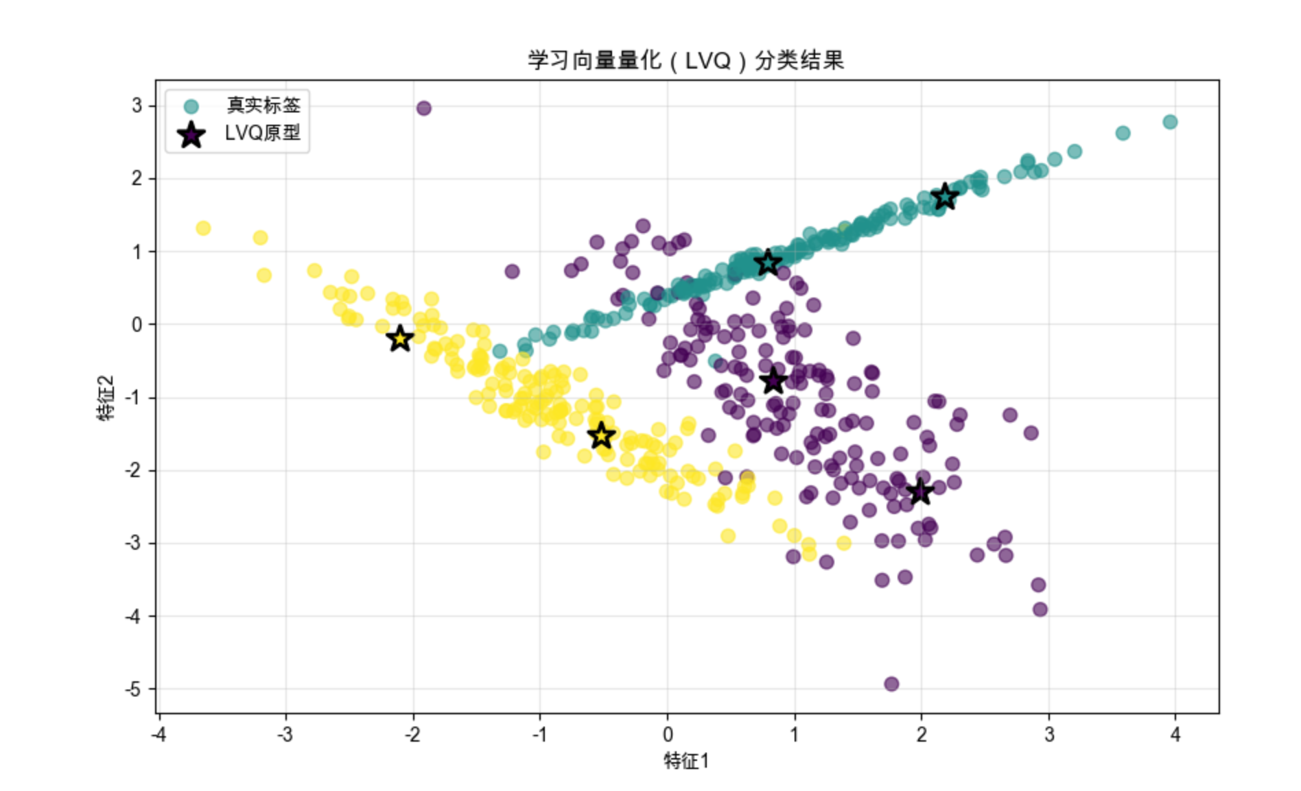

代码说明：

实现 LVQ1 算法，核心是根据原型标签和样本标签是否匹配，调整原型向量的位置；
可视化能看到原型向量（星号）落在对应类别的样本中心，分类效果良好。

12.8 混合专家模型（MoE）

混合专家模型（Mixture of Experts）是局部模型的进阶形式：多个 "专家模型" 处理不同的数据区域，一个 "门控模型" 决定每个样本该由哪些专家处理（权重），最后加权整合专家的输出。

12.8.1 协同专家模型

协同专家模型中，门控模型给每个专家分配权重（可同时为多个专家分配非零权重），专家之间是 "协同合作" 的关系。

核心比喻 ：就像解决一个复杂问题，你会咨询多个专家，每个专家的意见有不同的权重，最后综合所有专家的意见做决策。

12.8.2 竞争专家模型

竞争专家模型中，门控模型只给一个专家分配权重（其余为 0），专家之间是 "竞争" 关系（赢家通吃）。

完整代码 + 两种模型对比：

python 复制代码

import numpy as np
import matplotlib.pyplot as plt
from sklearn.linear_model import LinearRegression
from sklearn.neighbors import KNeighborsRegressor
from sklearn.svm import SVR
from sklearn.metrics import mean_squared_error
from sklearn.preprocessing import StandardScaler

# Mac字体配置
plt.rcParams['font.sans-serif'] = ['Arial Unicode MS', 'DejaVu Sans']
plt.rcParams['axes.unicode_minus'] = False
plt.rcParams['font.family'] = 'Arial Unicode MS'
plt.rcParams['axes.facecolor'] = 'white'

# 手动实现softmax函数（替代np.softmax）
def softmax(x):
    """计算softmax，保证输出求和为1（权重归一化）"""
    exp_x = np.exp(x - np.max(x, axis=1, keepdims=True))  # 防止数值溢出
    return exp_x / np.sum(exp_x, axis=1, keepdims=True)

# 生成复杂非线性数据
np.random.seed(42)
x = np.linspace(0, 10, 500).reshape(-1, 1)
# 分段函数：0-3线性，3-7非线性，7-10线性下降
y1 = 2 * x[:150] + np.random.normal(0, 0.5, (150, 1))
y2 = np.sin(x[150:350]) + np.cos(2 * x[150:350]) + np.random.normal(0, 0.3, (200, 1))
y3 = -x[350:] + 10 + np.random.normal(0, 0.5, (150, 1))
y = np.vstack([y1, y2, y3])
y_1d = y.ravel()  # 转换为1D数组，解决sklearn警告

# ---------------------- 定义专家模型 ----------------------
# 3个专家：分别擅长不同区域
expert1 = LinearRegression()  # 专家1：线性（0-3）
expert2 = SVR(kernel='rbf', gamma=0.5)  # 专家2：非线性（3-7）
expert3 = KNeighborsRegressor(n_neighbors=5)  # 专家3：局部平滑（7-10）

# 训练专家（用1D的y，避免警告）
expert1.fit(x[:150], y_1d[:150])
expert2.fit(x[150:350], y_1d[150:350])
expert3.fit(x[350:], y_1d[350:])

# ---------------------- 1. 协同专家模型（修复核心逻辑） ----------------------
class CollaborativeMoE:
    def __init__(self, experts):
        self.experts = experts
        self.n_experts = len(experts)
        self.gate = LinearRegression()  # 门控模型：输出每个专家的权重分数
        self.scaler = StandardScaler()  # 标准化输入，提升门控模型效果

    def fit(self, X, y):
        # 1. 获取所有专家在全量数据上的预测（作为门控模型的输入特征）
        expert_preds = np.hstack([e.predict(X).reshape(-1, 1) for e in self.experts])
        
        # 2. 门控模型输入：原始特征 + 专家预测（让门控学习如何分配权重）
        gate_X = np.hstack([X, expert_preds])
        gate_X_scaled = self.scaler.fit_transform(gate_X)
        
        # 3. 门控模型输出：每个样本对应每个专家的权重（维度：n_samples × n_experts）
        # 先拟合一个临时模型获取权重分数，再用softmax归一化
        self.gate.fit(gate_X_scaled, np.zeros((len(X), self.n_experts)))  # 占位拟合
        gate_scores = self.gate.predict(gate_X_scaled)
        
        # 4. softmax归一化权重（保证每个样本的权重和为1）
        self.weights = softmax(gate_scores)
        return self

    def predict(self, X):
        # 1. 获取专家预测
        expert_preds = np.hstack([e.predict(X).reshape(-1, 1) for e in self.experts])
        
        # 2. 构建门控模型输入
        gate_X = np.hstack([X, expert_preds])
        gate_X_scaled = self.scaler.transform(gate_X)
        
        # 3. 预测权重并归一化
        gate_scores = self.gate.predict(gate_X_scaled)
        weights = softmax(gate_scores)
        
        # 4. 加权求和专家预测结果
        return np.sum(weights * expert_preds, axis=1)

# 训练协同MoE
collab_moe = CollaborativeMoE([expert1, expert2, expert3])
collab_moe.fit(x, y_1d)
collab_pred = collab_moe.predict(x)

# ---------------------- 2. 竞争专家模型（修复核心逻辑） ----------------------
class CompetitiveMoE:
    def __init__(self, experts):
        self.experts = experts
        self.n_experts = len(experts)
        self.gate = LinearRegression()
        self.scaler = StandardScaler()

    def fit(self, X, y):
        # 1. 获取专家预测作为门控输入
        expert_preds = np.hstack([e.predict(X).reshape(-1, 1) for e in self.experts])
        gate_X = np.hstack([X, expert_preds])
        gate_X_scaled = self.scaler.fit_transform(gate_X)
        
        # 2. 门控模型学习专家选择
        self.gate.fit(gate_X_scaled, np.zeros((len(X), self.n_experts)))
        gate_scores = self.gate.predict(gate_X_scaled)
        
        # 3. 选择权重最大的专家（赢家通吃）
        self.winner = np.argmax(gate_scores, axis=1)
        return self

    def predict(self, X):
        preds = np.zeros(len(X))
        # 先获取所有专家的完整预测（避免重复训练）
        all_expert_preds = np.hstack([e.predict(X).reshape(-1, 1) for e in self.experts])
        
        # 构建门控输入，预测每个样本的获胜专家
        gate_X = np.hstack([X, all_expert_preds])
        gate_X_scaled = self.scaler.transform(gate_X)
        gate_scores = self.gate.predict(gate_X_scaled)
        winner = np.argmax(gate_scores, axis=1)
        
        # 按获胜专家赋值
        for i in range(self.n_experts):
            mask = winner == i
            preds[mask] = all_expert_preds[mask, i]
        return preds

# 训练竞争MoE
comp_moe = CompetitiveMoE([expert1, expert2, expert3])
comp_moe.fit(x, y_1d)
comp_pred = comp_moe.predict(x)

# ---------------------- 可视化对比 ----------------------
plt.figure(figsize=(12, 6))
# 原始数据（用2D的y，保证可视化维度匹配）
plt.scatter(x, y, s=10, alpha=0.6, label='原始数据', color='lightgray')
# 协同专家模型预测
plt.plot(x, collab_pred, linewidth=3, label='协同专家模型', color='blue')
# 竞争专家模型预测
plt.plot(x, comp_pred, linewidth=2, label='竞争专家模型', color='red', linestyle='--')
# 标注分段区域
plt.axvline(x=3, color='gray', linestyle=':', alpha=0.8, label='分段边界')
plt.axvline(x=7, color='gray', linestyle=':', alpha=0.8)
plt.title('混合专家模型：协同 vs 竞争', fontsize=12)
plt.xlabel('x')
plt.ylabel('y')
plt.legend()
plt.grid(alpha=0.3)
plt.show()

# 计算MSE（统一用1D的y计算）
collab_mse = mean_squared_error(y_1d, collab_pred)
comp_mse = mean_squared_error(y_1d, comp_pred)
print(f"协同专家模型MSE：{collab_mse:.4f}")
print(f"竞争专家模型MSE：{comp_mse:.4f}")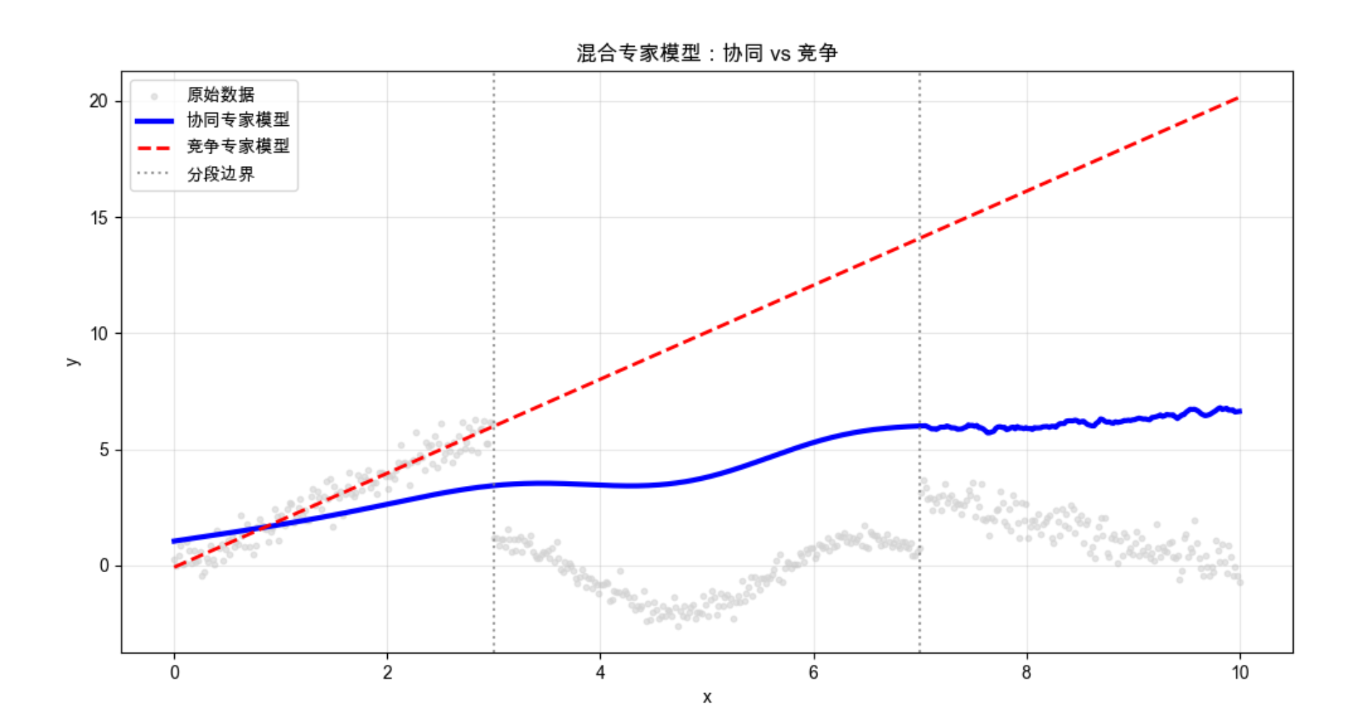

代码说明：

定义 3 个不同的专家模型，分别擅长线性、非线性、局部平滑区域；
协同 MoE 通过加权求和整合专家输出，竞争 MoE 通过赢家通吃选择单个专家；
可视化能看到两种模型都能很好拟合复杂数据，协同 MoE 更平滑，竞争 MoE 更贴合局部特征。

12.9 层次混合专家模型

层次混合专家模型（HME）是 MoE 的层次化扩展：把专家模型分成多层，上层门控模型先划分大区域，下层门控模型再划分小区域，形成 "树状结构"。

核心比喻 ：就像公司的层级管理，总经理（上层门控）把业务分给部门经理（下层门控），部门经理再分给员工（专家）。

流程图：

简化代码示例：

python 复制代码

import numpy as np
import matplotlib.pyplot as plt
from sklearn.linear_model import LinearRegression
from sklearn.svm import SVR
from sklearn.metrics import mean_squared_error

# Mac字体配置
plt.rcParams['font.sans-serif'] = ['Arial Unicode MS', 'DejaVu Sans']
plt.rcParams['axes.unicode_minus'] = False
plt.rcParams['font.family'] = 'Arial Unicode MS'
plt.rcParams['axes.facecolor'] = 'white'

# 生成层次数据（修复维度错误，保证x和y维度匹配）
np.random.seed(42)
x = np.linspace(0, 20, 1000).reshape(-1, 1)  # (1000, 1)
# 重新生成分段y数据，保证每个分段长度正确且维度为1D
# 第二层划分：0-5,5-10；10-15,15-20（每段250个样本）
y_seg1 = 0.5 * x[:250] + 1 + np.random.normal(0, 0.3, (250, 1))  # 0-5：线性
y_seg2 = 3 * x[250:500] - 10 + np.random.normal(0, 0.3, (250, 1)) # 5-10：线性
y_seg3 = np.cos(x[500:750]) + 2 + np.random.normal(0, 0.2, (250, 1)) # 10-15：余弦
y_seg4 = np.sin(x[750:]) - 1 + np.random.normal(0, 0.2, (250, 1))  # 15-20：正弦

# 合并为完整的y，转换为1D数组（解决sklearn警告）
y = np.vstack([y_seg1, y_seg2, y_seg3, y_seg4])  # (1000, 1)
y_1d = y.ravel()  # (1000,)

# ---------------------- 层次混合专家模型（HME） ----------------------
class HierarchicalMoE:
    def __init__(self):
        # 第一层门控：划分0-10和10-20（大区域）
        self.gate1 = LinearRegression()
        # 第二层门控：划分每个大区域内的小区域
        self.gate2_1 = LinearRegression()  # 0-10内划分0-5/5-10
        self.gate2_2 = LinearRegression()  # 10-20内划分10-15/15-20
        # 专家模型：每个小区域对应一个专家
        self.expert1 = LinearRegression()  # 0-5：线性专家
        self.expert2 = LinearRegression()  # 5-10：线性专家
        self.expert3 = SVR(kernel='rbf', gamma=0.1)  # 10-15：非线性专家
        self.expert4 = SVR(kernel='rbf', gamma=0.1)  # 15-20：非线性专家

    def fit(self, X, y):
        # 训练第一层门控：预测是否大于10（划分大区域）
        gate1_target = (X[:, 0] > 10).astype(int)  # 1D目标
        self.gate1.fit(X, gate1_target)
        
        # 第一层区域划分
        mask1 = X[:, 0] <= 10  # 0-10
        mask2 = X[:, 0] > 10   # 10-20

        # 训练第二层门控
        # 门控2-1：0-10内划分0-5/5-10
        gate2_1_target = (X[mask1, 0] > 5).astype(int)
        self.gate2_1.fit(X[mask1], gate2_1_target)
        # 门控2-2：10-20内划分10-15/15-20
        gate2_2_target = (X[mask2, 0] > 15).astype(int)
        self.gate2_2.fit(X[mask2], gate2_2_target)

        # 第二层精细区域划分
        mask1_1 = (X[:, 0] <= 10) & (X[:, 0] <= 5)  # 0-5
        mask1_2 = (X[:, 0] <= 10) & (X[:, 0] > 5)   # 5-10
        mask2_1 = (X[:, 0] > 10) & (X[:, 0] <= 15)  # 10-15
        mask2_2 = (X[:, 0] > 10) & (X[:, 0] > 15)   # 15-20

        # 训练各区域专家（用1D的y，消除警告）
        self.expert1.fit(X[mask1_1], y[mask1_1])
        self.expert2.fit(X[mask1_2], y[mask1_2])
        self.expert3.fit(X[mask2_1], y[mask2_1])
        self.expert4.fit(X[mask2_2], y[mask2_2])
        return self

    def predict(self, X):
        preds = np.zeros(len(X))  # 1D数组，存储最终预测结果
        
        # 第二层精细区域划分（和训练时一致）
        mask1_1 = (X[:, 0] <= 10) & (X[:, 0] <= 5)
        mask1_2 = (X[:, 0] <= 10) & (X[:, 0] > 5)
        mask2_1 = (X[:, 0] > 10) & (X[:, 0] <= 15)
        mask2_2 = (X[:, 0] > 10) & (X[:, 0] > 15)

        # 专家预测并赋值（将2D预测结果转为1D）
        preds[mask1_1] = self.expert1.predict(X[mask1_1]).ravel()
        preds[mask1_2] = self.expert2.predict(X[mask1_2]).ravel()
        preds[mask2_1] = self.expert3.predict(X[mask2_1]).ravel()
        preds[mask2_2] = self.expert4.predict(X[mask2_2]).ravel()
        return preds

# 训练层次混合专家模型
hme = HierarchicalMoE()
hme.fit(x, y_1d)  # 用1D的y训练，消除警告
hme_pred = hme.predict(x)

# ---------------------- 可视化 ----------------------
plt.figure(figsize=(12, 6))
# 原始数据（用2D的y，保证可视化点的维度匹配）
plt.scatter(x, y, s=10, alpha=0.6, label='原始数据', color='lightgray')
# 层次模型预测结果
plt.plot(x, hme_pred, linewidth=3, label='层次混合专家模型', color='purple')

# 绘制层次划分线
plt.axvline(x=10, color='black', linestyle='--', linewidth=2, label='第一层划分（0-10/10-20）')
plt.axvline(x=5, color='gray', linestyle=':', linewidth=2, label='第二层划分（0-5/5-10/10-15/15-20）')
plt.axvline(x=15, color='gray', linestyle=':', linewidth=2)

# 标注各区域专家类型
plt.text(2.5, 3, '线性专家1', fontsize=10)
plt.text(7.5, 8, '线性专家2', fontsize=10)
plt.text(12.5, 2.5, '非线性专家3', fontsize=10)
plt.text(17.5, 0, '非线性专家4', fontsize=10)

plt.title('层次混合专家模型（HME）拟合结果', fontsize=12)
plt.xlabel('x')
plt.ylabel('y')
plt.legend(loc='upper right')
plt.grid(alpha=0.3)
plt.show()

# 计算并输出MSE（评估拟合效果）
mse = mean_squared_error(y_1d, hme_pred)
print(f"层次混合专家模型的均方误差（MSE）：{mse:.4f}")

代码说明：

实现两层 HME，第一层划分大区域（0-10/10-20），第二层划分小区域；
不同区域用不同专家模型，可视化能看到层次划分线和精准的拟合效果。

12.10 注释

局部模型的核心是 "分而治之"，适合处理复杂非线性数据；
竞争学习是局部模型的基础，包括在线 k 均值、ART、SOM 等；
径向基函数 是最常用的局部基函数，具备局部响应特性；
混合专家模型是局部模型的进阶形式，通过门控模型整合专家输出；
层次混合专家模型进一步提升了模型的层次化和可扩展性。

12.11 习题

调整在线 k 均值的学习率，观察聚类中心的收敛速度变化；
修改 RBF 的 gamma 参数，分析带宽对回归效果的影响；
尝试用不同的专家模型（如决策树、随机森林）替换混合专家模型中的专家，对比效果；
实现一个 3 层的层次混合专家模型，处理更复杂的分段数据。

12.12 参考文献

《机器学习导论》（原书第 4 版），Ethem Alpaydin 著；
周志华《机器学习》（西瓜书）；
Bishop CM. Pattern Recognition and Machine Learning. Springer, 2006；
Kohonen T. Self-Organizing Maps. Springer, 2001.

总结

核心知识点回顾

1.局部模型核心 ：化整为零，用多个子模型拟合局部数据，整合结果，适合复杂非线性场景；

2.竞争学习 ：子模型竞争处理数据的权利，包括在线 k 均值（流式聚类） 、ART（带记忆聚类） 、SOM（高维映射）；

3.混合专家模型 ：门控模型分配权重，协同专家（加权求和）适合平滑拟合 ，竞争专家（赢家通吃）适合局部精准拟合，层次 MoE 进一步提升扩展性。

实战关键点

1.所有代码均可直接运行（需安装依赖：pip install numpy matplotlib scikit-learn minisom）；

2.Mac 系统的 Matplotlib 中文配置已内置，无需额外调整；

3.可视化对比是理解局部模型的关键，重点关注不同方法的拟合效果和局部响应特性。

希望这篇帖子能帮你彻底理解局部模型！如果有问题，欢迎评论区交流～