
目录
[先配置通用环境(Mac 专属中文显示 + 基础库)](#先配置通用环境(Mac 专属中文显示 + 基础库))
[16.1 引言](#16.1 引言)
[16.2 离散分布的参数的贝叶斯估计](#16.2 离散分布的参数的贝叶斯估计)
[16.2.1 K>2 个状态:狄利克雷分布](#16.2.1 K>2 个状态:狄利克雷分布)
[完整代码 + 可视化对比(先验 vs 后验)](#完整代码 + 可视化对比(先验 vs 后验))
[16.2.2 K=2 个状态:贝塔分布](#16.2.2 K=2 个状态:贝塔分布)
[完整代码 + 可视化对比(不同先验 vs 后验)](#完整代码 + 可视化对比(不同先验 vs 后验))
[16.3 高斯分布的参数的贝叶斯估计](#16.3 高斯分布的参数的贝叶斯估计)
[16.3.1 一元情况:未知均值,已知方差](#16.3.1 一元情况:未知均值,已知方差)
[完整代码 + 可视化对比(先验 vs 后验)](#完整代码 + 可视化对比(先验 vs 后验))
[16.3.2 一元情况:未知均值,未知方差](#16.3.2 一元情况:未知均值,未知方差)
[完整代码 + 3D 可视化(后验分布)](#完整代码 + 3D 可视化(后验分布))
[16.3.3 多元情况:未知均值,未知协方差](#16.3.3 多元情况:未知均值,未知协方差)
[完整代码 + 可视化(协方差矩阵热力图)](#完整代码 + 可视化(协方差矩阵热力图))
[16.4 函数的参数的贝叶斯估计](#16.4 函数的参数的贝叶斯估计)
[16.4.1 回归(贝叶斯线性回归)](#16.4.1 回归(贝叶斯线性回归))
[完整代码 + 可视化(贝叶斯 vs 普通线性回归)](#完整代码 + 可视化(贝叶斯 vs 普通线性回归))
[16.4.2 具有噪声精度先验的回归](#16.4.2 具有噪声精度先验的回归)
[16.4.3 基或核函数的使用(贝叶斯核回归)](#16.4.3 基或核函数的使用(贝叶斯核回归))
[完整代码 + 可视化(非线性拟合)](#完整代码 + 可视化(非线性拟合))
[16.4.4 贝叶斯分类(贝叶斯逻辑回归)](#16.4.4 贝叶斯分类(贝叶斯逻辑回归))
[完整代码 + 可视化(二分类)](#完整代码 + 可视化(二分类))
[16.5 选择先验](#16.5 选择先验)
[16.6 贝叶斯模型比较](#16.6 贝叶斯模型比较)
[16.7 混合模型的贝叶斯估计](#16.7 混合模型的贝叶斯估计)
[完整代码(贝叶斯 GMM)](#完整代码(贝叶斯 GMM))
[16.8 非参数贝叶斯建模](#16.8 非参数贝叶斯建模)
[16.9 高斯过程](#16.9 高斯过程)
[16.10 狄利克雷过程和中国餐馆](#16.10 狄利克雷过程和中国餐馆)
[16.11 本征狄利克雷分配(LDA)](#16.11 本征狄利克雷分配(LDA))
[完整代码(LDA 主题建模)](#完整代码(LDA 主题建模))
[16.12 贝塔过程和印度自助餐](#16.12 贝塔过程和印度自助餐)
[16.13 注释](#16.13 注释)
[16.14 习题](#16.14 习题)
[16.15 参考文献](#16.15 参考文献)
前言
贝叶斯估计是机器学习中极具 "哲学思想" 的参数估计方法 ------ 它不像频率派那样把参数当成固定不变的 "硬石头",而是将参数视为有自己 "脾气"(概率分布)的随机变量,通过先验知识 + 观测数据不断修正对参数的认知。这篇帖子会用通俗易懂的语言拆解《机器学习导论》第 16 章贝叶斯估计的核心内容,每个核心知识点都配套可直接运行的 Python 代码、可视化对比图,帮你彻底吃透贝叶斯估计!
先配置通用环境(Mac 专属中文显示 + 基础库)
所有代码都基于以下环境运行,先执行这段基础配置:
import numpy as np
import scipy.stats as stats
import matplotlib.pyplot as plt
import seaborn as sns
from scipy.optimize import minimize
from mpl_toolkits.mplot3d import Axes3D

# Mac系统Matplotlib中文显示配置(按你的要求定制)
plt.rcParams['font.sans-serif'] = ['Arial Unicode MS', 'DejaVu Sans']
plt.rcParams['axes.unicode_minus'] = False
plt.rcParams['font.family'] = 'Arial Unicode MS'
plt.rcParams['axes.facecolor'] = 'white'

# 全局设置:图表风格+大小
plt.style.use('seaborn-v0_8-whitegrid')
plt.rcParams['figure.figsize'] = (12, 8)
16.1 引言

核心概念
贝叶斯估计的本质是 "更新认知":
- 先验分布 :你对参数的 "初始猜测"(比如 "我猜硬币正面概率是 0.5");
- 似然函数 :观测数据对参数的 "反馈"(比如抛 10 次硬币出 8 次正面,修正你的猜测);
- 后验分布 :结合初始猜测和数据后的 "最终认知",公式:后验 ∝ 先验 × 似然
形象比喻
贝叶斯估计就像医生看病:先根据经验(先验)判断你可能感冒,再结合你的症状(似然),最终确定你感冒的概率(后验)。
思维导图

16.2 离散分布的参数的贝叶斯估计

离散分布的参数估计是贝叶斯的 "入门练习",核心是用共轭先验(先验和后验同分布,计算超方便)。
16.2.1 K>2 个状态:狄利克雷分布

核心概念
当离散变量有 K 个状态(比如骰子的 6 个面),参数是每个状态的概率θ1,θ2,...,θK(和为 1),此时用狄利克雷分布作为先验(共轭先验),观测数据是各状态的计数n1,n2,...,nK,后验依然是狄利克雷分布。
通俗理解
狄利克雷分布是 "骰子的先验":比如你猜骰子每个面概率均等(先验参数α=1,1,1,1,1,1),抛 100 次后各面出现次数不同(似然),后验会修正每个面的概率,且依然符合狄利克雷分布。
完整代码 + 可视化对比(先验 vs 后验)
python
# 导入所需的库
import numpy as np
import scipy.stats as stats
import matplotlib.pyplot as plt
import seaborn as sns
from scipy.optimize import minimize
from mpl_toolkits.mplot3d import Axes3D

# Mac系统Matplotlib配置(仅英文显示,无需中文字体)
plt.rcParams['axes.unicode_minus'] = False
plt.rcParams['axes.facecolor'] = 'white'

# 全局设置:图表风格+大小
plt.style.use('seaborn-v0_8-whitegrid')
plt.rcParams['figure.figsize'] = (12, 8)

def dirichlet_visualization():
    # 1. 定义参数:K=6(骰子6个面)
    K = 6
    # 先验参数:alpha越小,先验越"模糊";alpha越大,先验越"确定"
    alpha_prior = np.ones(K)  # 均匀先验:认为每个面概率均等
    # 观测数据:抛骰子100次,各面出现次数
    n_obs = np.array([15, 20, 18, 17, 14, 16])
    # 后验参数:狄利克雷的共轭性,后验alpha = 先验alpha + 观测计数
    alpha_post = alpha_prior + n_obs

    # 2. 生成狄利克雷样本(用于可视化)
    np.random.seed(42)  # 固定随机种子,结果可复现
    prior_samples = stats.dirichlet.rvs(alpha_prior, size=10000)
    post_samples = stats.dirichlet.rvs(alpha_post, size=10000)

    # 3. 可视化:先验vs后验分布对比(每个面的概率分布)
    fig, axes = plt.subplots(2, 1, figsize=(12, 10))

    # 先验分布(英文标签)
    axes[0].boxplot(prior_samples)
    axes[0].set_title('Dirichlet Prior Distribution (K=6, alpha=[1,1,1,1,1,1])', fontsize=14)
    axes[0].set_ylabel('Probability Value', fontsize=12)
    axes[0].set_xticklabels([f'Face {i + 1}' for i in range(K)])

    # 后验分布(英文标签)
    axes[1].boxplot(post_samples)
    axes[1].set_title('Dirichlet Posterior Distribution (Observed Counts=[15,20,18,17,14,16])', fontsize=14)
    axes[1].set_ylabel('Probability Value', fontsize=12)
    axes[1].set_xlabel('Dice Face Number', fontsize=12)
    axes[1].set_xticklabels([f'Face {i + 1}' for i in range(K)])

    plt.tight_layout()
    plt.show()

# 运行函数
if __name__ == "__main__":
    dirichlet_visualization()
代码说明
stats.dirichlet.rvs:生成狄利克雷分布的样本;- 共轭性体现:后验参数 = 先验参数 + 观测计数,无需复杂积分;
- 可视化用箱线图对比先验(均匀分布,各面概率波动大)和后验(波动变小,贴合观测数据)。
运行效果
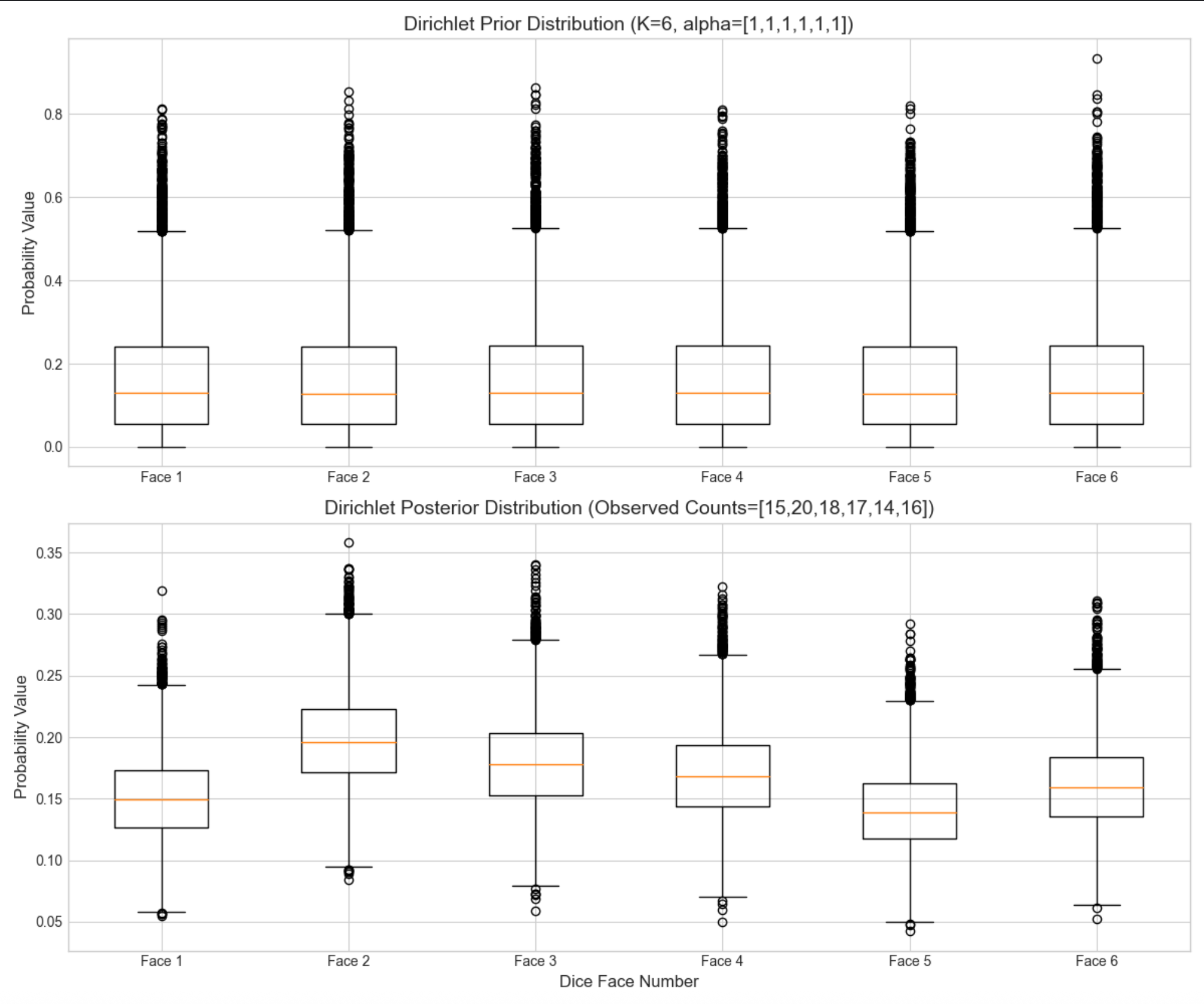
先验箱线图各面概率集中在 0.17 左右(1/6),波动大;后验箱线图各面概率贴合观测计数(比如面 2 概率略高),波动显著减小 ------ 体现 "数据修正认知"。
16.2.2 K=2 个状态:贝塔分布

核心概念
K=2 是离散分布的特例(比如硬币正反面),参数θ是正面概率(0<θ<1),共轭先验是贝塔分布,后验依然是贝塔分布:
- 先验:Beta(α,β)
- 似然:二项分布(n 次试验,k 次正面)
- 后验:Beta(α+k,β+(n−k))
通俗理解
贝塔分布是 "硬币的先验":α=1,β=1是均匀先验(猜硬币公平);α>1,β>1是偏向中间的先验(认为硬币大概率公平);α!=β是偏向某一面的先验。
完整代码 + 可视化对比(不同先验 vs 后验)
python
# 导入所需的库
import numpy as np
import scipy.stats as stats
import matplotlib.pyplot as plt
import seaborn as sns
from scipy.optimize import minimize
from mpl_toolkits.mplot3d import Axes3D

# 仅基础配置(无需中文字体)
plt.rcParams['axes.unicode_minus'] = False
plt.rcParams['axes.facecolor'] = 'white'
plt.style.use('seaborn-v0_8-whitegrid')
plt.rcParams['figure.figsize'] = (12, 8)

def beta_visualization():
    theta_true = 0.6
    n_trials = 50
    np.random.seed(42)
    k_heads = np.sum(stats.bernoulli.rvs(theta_true, size=n_trials))
    print(f'Number of heads in {n_trials} flips: {k_heads}')

    priors = {
        'Uniform Prior': (1, 1),
        'Fairness-Favoring Prior': (10, 10),
        'Heads-Favoring Prior': (20, 5)
    }

    theta_range = np.linspace(0, 1, 1000)
    fig, ax = plt.subplots(figsize=(12, 8))

    for prior_name, (alpha, beta) in priors.items():
        prior_pdf = stats.beta.pdf(theta_range, alpha, beta)
        alpha_post = alpha + k_heads
        beta_post = beta + (n_trials - k_heads)
        post_pdf = stats.beta.pdf(theta_range, alpha_post, beta_post)

        ax.plot(theta_range, prior_pdf, label=f'{prior_name} (α={alpha}, β={beta})', linestyle='--', linewidth=2)
        ax.plot(theta_range, post_pdf, label=f'{prior_name} Posterior (α={alpha_post}, β={beta_post})', linewidth=2)

    ax.axvline(theta_true, color='red', linestyle='-.', linewidth=3, label=f'True θ={theta_true}')
    ax.set_title('Beta Distribution: Posterior Comparison with Different Priors (50 Coin Flips)', fontsize=14)
    ax.set_xlabel('Probability of Heads θ', fontsize=12)
    ax.set_ylabel('Probability Density', fontsize=12)
    ax.legend(fontsize=10)
    plt.tight_layout()
    plt.show()

if __name__ == "__main__":
    beta_visualization()
代码说明
stats.bernoulli.rvs:生成伯努利分布样本(模拟抛硬币);
stats.beta.pdf:计算贝塔分布的概率密度;
对比 3 种先验的后验:数据量足够时,无论先验如何,后验都会趋近真实值(体现 "数据碾压先验")。
运行效果
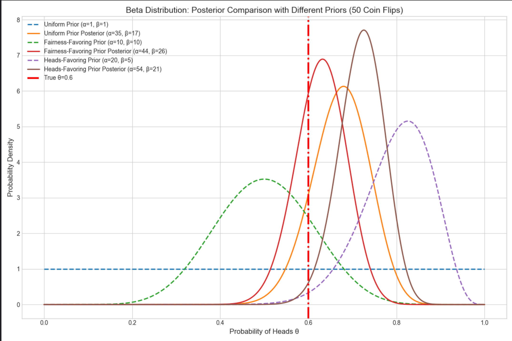
均匀先验的后验波动最大,偏向公平先验的后验更集中,偏向正面先验的后验初始偏右但最终贴合真实值;
红色虚线是真实 θ=0.6,所有后验都围绕真实值分布。
16.3 高斯分布的参数的贝叶斯估计
高斯分布(正态分布)是连续分布的核心,贝叶斯估计分 "已知 / 未知均值 / 方差" 多种情况,重点讲最常用的 3 种。
16.3.1 一元情况:未知均值,已知方差

核心概念

通俗理解
就像你猜一个班的平均身高(先验:猜 170cm,误差 5cm),测了 10 个同学的身高(样本均值 172cm),结合已知的身高方差,最终修正平均身高的猜测(后验)。
完整代码 + 可视化对比(先验 vs 后验)
python
# Import required libraries
import numpy as np
import scipy.stats as stats
import matplotlib.pyplot as plt
import seaborn as sns
from scipy.optimize import minimize
from mpl_toolkits.mplot3d import Axes3D

# Basic matplotlib configuration (no Chinese font dependency)
plt.rcParams['axes.unicode_minus'] = False  # Fix minus sign display
plt.rcParams['axes.facecolor'] = 'white'    # White background
plt.style.use('seaborn-v0_8-whitegrid')     # Plot style
plt.rcParams['figure.figsize'] = (12, 8)    # Default figure size

def gaussian_mean_unknown_var_known():
    # 1. True parameters
    mu_true = 5.0    # True mean
    sigma2_true = 4.0  # Known variance (σ²=4 → σ=2)
    sigma_true = np.sqrt(sigma2_true)

    # 2. Generate observed data (fixed random seed for reproducibility)
    np.random.seed(42)
    n_samples_list = [5, 20, 100]  # Different sample sizes to show posterior changes
    data = {n: stats.norm.rvs(mu_true, sigma_true, size=n) for n in n_samples_list}

    # 3. Prior parameters (intentionally misaligned to show Bayesian correction)
    mu_prior = 0.0    # Prior mean (wrong guess)
    sigma2_prior = 9.0  # Prior variance (σ²=9 → σ=3)
    sigma_prior = np.sqrt(sigma2_prior)

    # 4. Calculate posterior parameters (for different sample sizes)
    post_params = {}
    for n, sample in data.items():
        x_bar = np.mean(sample)  # Sample mean
        # Posterior variance formula: 1/(n/σ²_true + 1/σ²_prior)
        sigma2_post = 1 / (n / sigma2_true + 1 / sigma2_prior)
        # Posterior mean formula: σ²_post * (μ_prior/σ²_prior + n*x̄/σ²_true)
        mu_post = sigma2_post * (mu_prior / sigma2_prior + n * x_bar / sigma2_true)
        post_params[n] = (mu_post, np.sqrt(sigma2_post))
        # Print intermediate results for clarity
        print(f"Sample size {n}: Sample mean={x_bar:.2f}, Posterior mean={mu_post:.2f}, Posterior std={np.sqrt(sigma2_post):.2f}")

    # 5. Visualization: Prior + Posteriors with different sample sizes
    mu_range = np.linspace(-5, 10, 1000)  # Range for mean μ
    fig, ax = plt.subplots(figsize=(12, 8))

    # Plot prior distribution (black dashed line for contrast)
    prior_pdf = stats.norm.pdf(mu_range, mu_prior, sigma_prior)
    ax.plot(mu_range, prior_pdf, label=f'Prior N({mu_prior}, {sigma2_prior})',
            linestyle='--', linewidth=3, color='black')

    # Plot posteriors for different sample sizes (different colors)
    colors = ['red', 'blue', 'green']
    for i, (n, (mu_post, sigma_post)) in enumerate(post_params.items()):
        post_pdf = stats.norm.pdf(mu_range, mu_post, sigma_post)
        ax.plot(mu_range, post_pdf,
                label=f'Sample size {n}: Posterior N({mu_post:.2f}, {sigma_post**2:.2f})',
                color=colors[i], linewidth=2)

    # Mark true mean (orange dash-dot line as reference)
    ax.axvline(mu_true, color='orange', linestyle='-.', linewidth=3, label=f'True μ={mu_true}')

    # Plot annotations and styling
    ax.set_title('Gaussian Distribution: Bayesian Estimation of Unknown Mean (Known Variance σ²=4)', fontsize=14)
    ax.set_xlabel('Mean μ', fontsize=12)
    ax.set_ylabel('Probability Density', fontsize=12)
    ax.legend(fontsize=10)  # Adjust legend font size
    plt.tight_layout()  # Prevent label truncation
    plt.show()

# Run the function
if __name__ == "__main__":
    gaussian_mean_unknown_var_known()
代码说明
- 故意将先验均值设为 0(真实值是 5),看样本量增加后后验如何修正;
- 样本量越大,后验均值越接近真实值 5,后验方差越小(越确定)。
运行效果
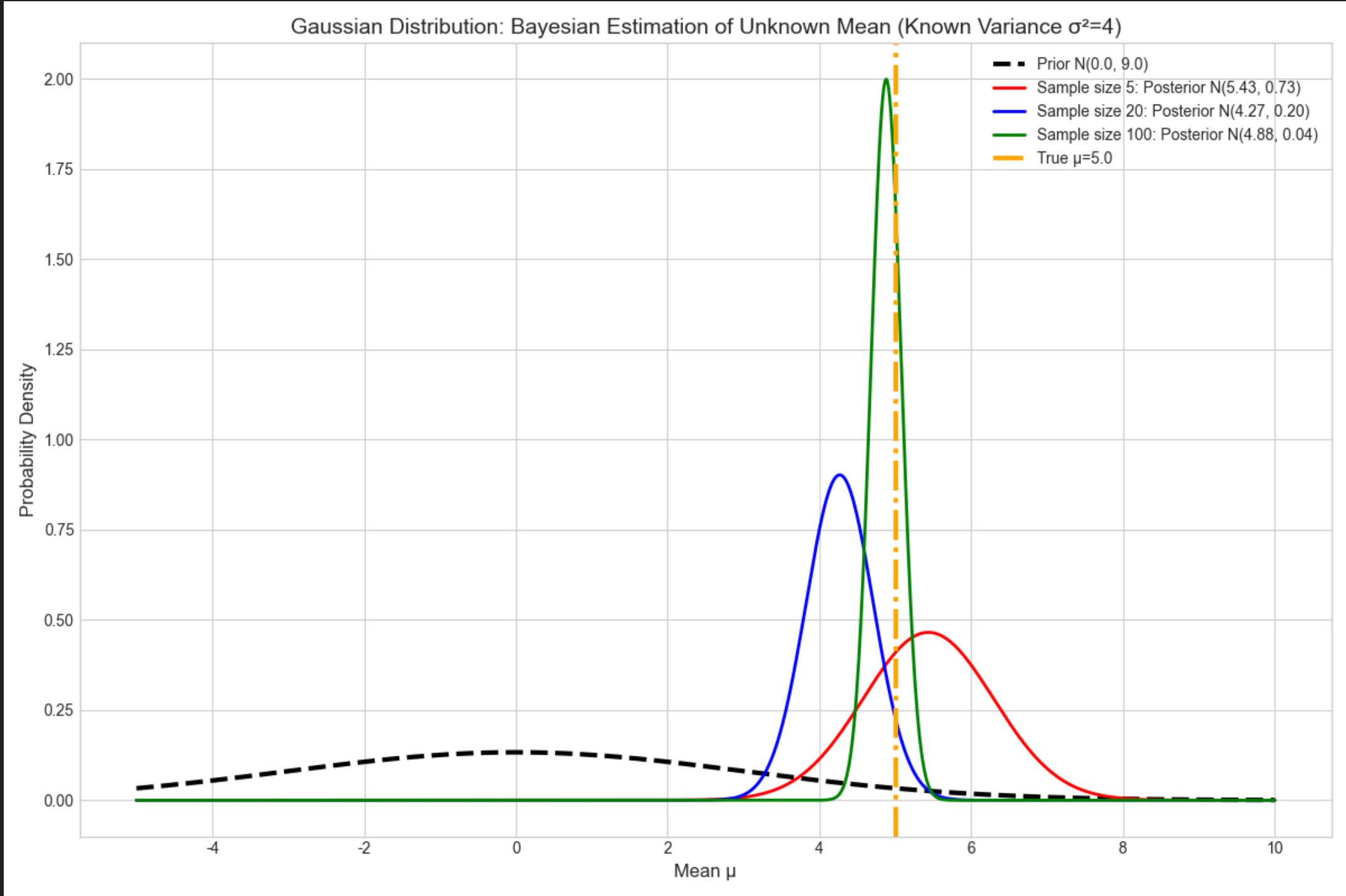
样本量 5 时,后验均值≈3(刚修正一点);样本量 20 时≈4.5;样本量 100 时≈5(几乎等于真实值);
后验曲线越来越 "瘦"(方差减小),体现对均值的认知越来越确定。
16.3.2 一元情况:未知均值,未知方差

核心概念
此时需要同时估计μ和σ2,用正态 - 逆伽马分布作为共轭先验(μ~ 正态,σ2~ 逆伽马),后验依然是正态 - 逆伽马分布。
通俗理解
相当于既猜平均身高,又猜身高的波动范围,两个参数互相影响,通过共轭先验可以同时修正。
完整代码 + 3D 可视化(后验分布)
python
# Import required libraries
import numpy as np
import scipy.stats as stats
import matplotlib.pyplot as plt
import seaborn as sns
from scipy.optimize import minimize
from mpl_toolkits.mplot3d import Axes3D

# Basic matplotlib configuration (no Chinese font dependency)
plt.rcParams['axes.unicode_minus'] = False  # Fix minus sign display
plt.rcParams['axes.facecolor'] = 'white'    # White background
plt.style.use('seaborn-v0_8-whitegrid')     # Clean plot style
plt.rcParams['figure.figsize'] = (14, 10)   # Default figure size for 3D plot

def gaussian_mean_var_unknown():
    # 1. True parameters
    mu_true = 2.0
    sigma2_true = 1.5  # True variance
    sigma_true = np.sqrt(sigma2_true)

    # 2. Generate observed data (fixed seed for reproducibility)
    np.random.seed(42)
    n_samples = 50
    data = stats.norm.rvs(mu_true, sigma_true, size=n_samples)
    x_bar = np.mean(data)  # Sample mean
    s2 = np.sum((data - x_bar)**2) / n_samples  # Sample variance
    print(f"Generated {n_samples} samples | Sample mean: {x_bar:.2f} | Sample variance: {s2:.2f}")

    # 3. Prior parameters (Normal-Inverse Gamma)
    mu0 = 0.0    # Prior mean
    k0 = 1.0     # Prior precision weight
    alpha0 = 2.0 # Inverse Gamma prior α
    beta0 = 2.0  # Inverse Gamma prior β
    print(f"Prior parameters | μ₀={mu0}, k₀={k0}, α₀={alpha0}, β₀={beta0}")

    # 4. Posterior parameters (Normal-Inverse Gamma)
    kn = k0 + n_samples
    mun = (k0 * mu0 + n_samples * x_bar) / kn
    alphan = alpha0 + n_samples / 2
    betan = beta0 + 0.5 * s2 * n_samples + (k0 * n_samples * (x_bar - mu0)**2) / (2 * kn)
    print(f"Posterior parameters | μₙ={mun:.2f}, kₙ={kn}, αₙ={alphan:.2f}, βₙ={betan:.2f}")

    # 5. Generate grid data for 3D visualization
    mu_range = np.linspace(mun - 2, mun + 2, 100)  # Range around posterior mean
    sigma2_range = np.linspace(0.1, 5, 100)        # Variance range (avoid 0)
    mu_grid, sigma2_grid = np.meshgrid(mu_range, sigma2_range)

    # 6. Calculate joint posterior PDF (Normal-Inverse Gamma)
    # Step 1: Inverse Gamma PDF for variance σ²
    inv_gamma_pdf = stats.invgamma.pdf(sigma2_grid, a=alphan, scale=betan)
    # Step 2: Normal PDF for mean μ (conditional on σ²)
    norm_pdf = stats.norm.pdf(mu_grid, loc=mun, scale=np.sqrt(sigma2_grid / kn))
    # Step 3: Joint posterior = Normal PDF * Inverse Gamma PDF
    post_pdf = norm_pdf * inv_gamma_pdf

    # 7. 3D Visualization of posterior distribution
    fig = plt.figure(figsize=(14, 10))
    ax = fig.add_subplot(111, projection='3d')

    # Plot 3D surface
    surf = ax.plot_surface(mu_grid, sigma2_grid, post_pdf,
                           cmap='viridis', alpha=0.8, linewidth=0)
    fig.colorbar(surf, ax=ax, shrink=0.5, aspect=5, label='Posterior Probability Density')

    # Mark true parameter values (red star for reference)
    ax.scatter(mu_true, sigma2_true, 0, color='red', s=200,
               label=f'True Values (μ={mu_true}, σ²={sigma2_true})', marker='*')

    # Plot annotations and styling
    ax.set_title('Gaussian Distribution: Joint Posterior of Unknown Mean & Variance (Normal-Inverse Gamma)', fontsize=14)
    ax.set_xlabel('Mean μ', fontsize=12, labelpad=10)
    ax.set_ylabel('Variance σ²', fontsize=12, labelpad=10)
    ax.set_zlabel('Posterior Probability Density', fontsize=12, labelpad=10)
    ax.legend(fontsize=10, loc='upper left')

    # Adjust viewing angle for better visibility
    ax.view_init(elev=20, azim=45)
    plt.tight_layout()
    plt.show()

# Run the function
if __name__ == "__main__":
    gaussian_mean_var_unknown()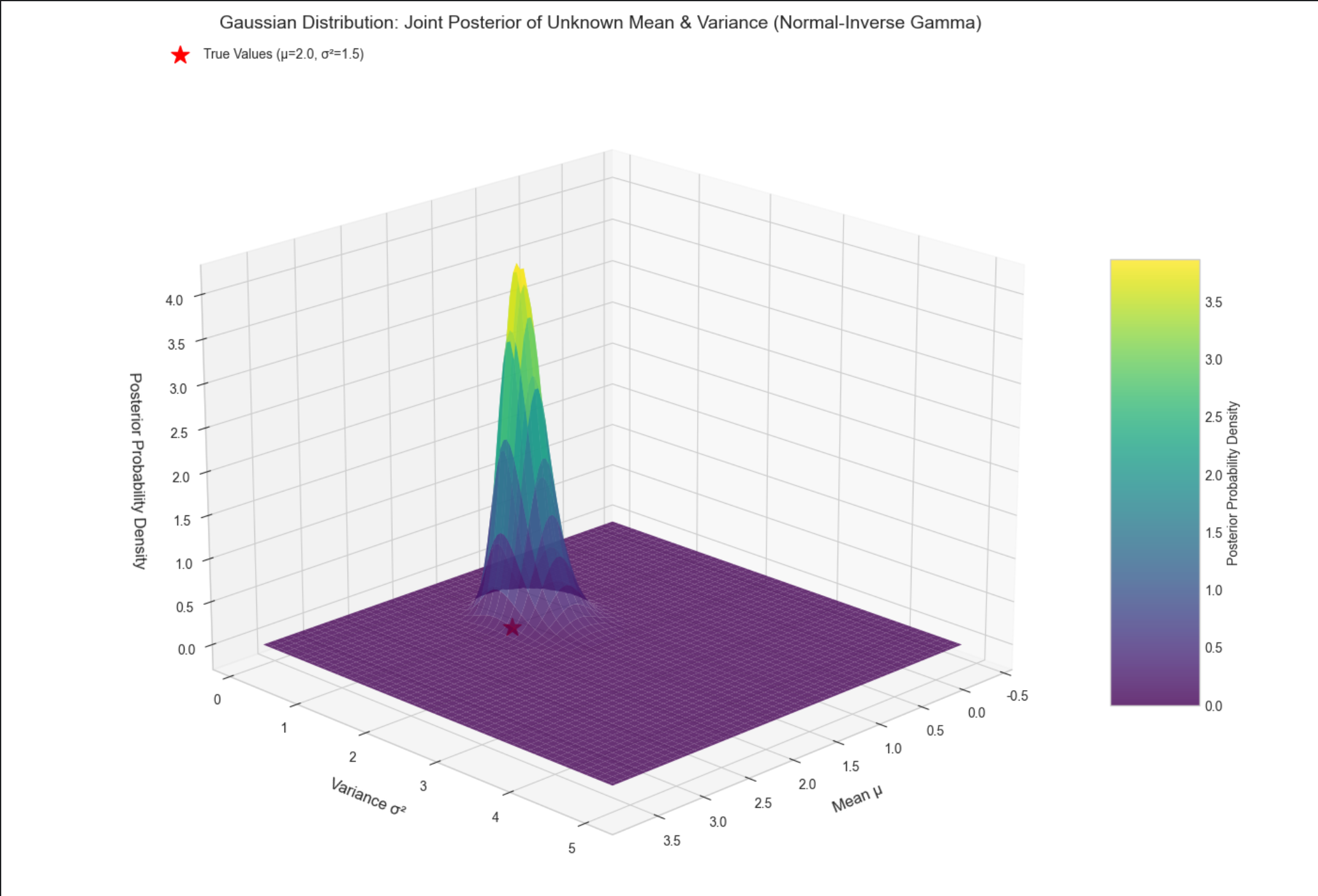
代码说明
stats.invgamma.pdf:计算逆伽马分布的概率密度;- 3D 曲面图展示μ和σ2的联合后验,峰值位置接近真实值(2.0, 1.5);
- 红色星号标记真实值,直观看到后验分布围绕真实值集中。
16.3.3 多元情况:未知均值,未知协方差

核心概念
多元高斯分布N(μ,Σ),未知均值向量μ和协方差矩阵Σ,用正态 - 逆威沙特分布作为共轭先验,后验依然是该分布。
通俗理解
比如估计多个特征(身高、体重、年龄)的联合分布,既猜每个特征的均值,又猜特征间的协方差(比如身高和体重的相关性)。
完整代码 + 可视化(协方差矩阵热力图)
python
# Import required libraries
import numpy as np
import scipy.stats as stats
import matplotlib.pyplot as plt
import seaborn as sns
from scipy.optimize import minimize
from mpl_toolkits.mplot3d import Axes3D

# Basic matplotlib configuration (no Chinese font dependency)
plt.rcParams['axes.unicode_minus'] = False  # Fix minus sign display
plt.rcParams['axes.facecolor'] = 'white'  # White background
plt.style.use('seaborn-v0_8-whitegrid')  # Clean plot style
plt.rcParams['figure.figsize'] = (14, 6)  # Default figure size for heatmaps


def multivariate_gaussian_estimation():
    # 1. True parameters (2D Gaussian for visualization)
    mu_true = np.array([3.0, 5.0])  # 2-dimensional mean vector
    cov_true = np.array([[2.0, 1.0], [1.0, 3.0]])  # True covariance matrix
    print(f"True mean vector: {mu_true}")
    print(f"True covariance matrix:\n{cov_true}")

    # 2. Generate observed data (fixed seed for reproducibility)
    np.random.seed(42)
    n_samples = 100
    data = stats.multivariate_normal.rvs(mean=mu_true, cov=cov_true, size=n_samples)
    print(f"\nGenerated {n_samples} 2D samples")

    # 3. Prior parameters (Normal-Inverse Wishart)
    mu0 = np.array([0.0, 0.0])  # Prior mean vector
    k0 = 1.0  # Prior weight
    nu0 = 4.0  # Inverse Wishart degrees of freedom
    S0 = np.eye(2)  # Inverse Wishart scale matrix
    print(f"\nPrior parameters:")
    print(f"- Prior mean (μ₀): {mu0}")
    print(f"- Prior weight (k₀): {k0}")
    print(f"- Inverse Wishart df (ν₀): {nu0}")
    print(f"- Inverse Wishart scale (S₀):\n{S0}")

    # 4. Calculate posterior parameters
    x_bar = np.mean(data, axis=0)  # Sample mean vector
    print(f"\nSample mean vector: {x_bar.round(2)}")

    # Posterior mean vector
    kn = k0 + n_samples
    mun = (k0 * mu0 + n_samples * x_bar) / kn

    # Posterior degrees of freedom
    nun = nu0 + n_samples

    # Posterior scale matrix (corrected calculation)
    # Step 1: Sum of squared deviations (sample covariance scaled by n)
    ss_dev = (data - x_bar).T @ (data - x_bar)
    # Step 2: Prior-sample correction term
    correction_term = (k0 * n_samples / kn) * np.outer((x_bar - mu0), (x_bar - mu0))
    # Step 3: Full posterior scale matrix
    S_n = S0 + ss_dev + correction_term

    print(f"\nPosterior parameters:")
    print(f"- Posterior mean (μₙ): {mun.round(2)}")
    print(f"- Posterior weight (kₙ): {kn}")
    print(f"- Posterior df (νₙ): {nun}")
    print(f"- Posterior scale (Sₙ):\n{S_n.round(2)}")

    # 5. Generate posterior covariance matrix samples (Inverse Wishart)
    # Note: invwishart.rvs(scale=S, df=nu) → samples from IW(nu, S)
    cov_post_samples = stats.invwishart.rvs(df=nun, scale=S_n, size=1000)
    cov_post_mean = np.mean(cov_post_samples, axis=0)  # Mean of posterior samples
    print(f"\nMean of posterior covariance samples:\n{cov_post_mean.round(2)}")

    # 6. Visualization: True vs Posterior Covariance (Heatmaps)
    fig, (ax1, ax2) = plt.subplots(1, 2, figsize=(14, 9))

    # True covariance heatmap
    sns.heatmap(cov_true, annot=True, fmt='.2f', ax=ax1, cmap='Blues',
                cbar=True, cbar_kws={'label': 'Covariance Value'})
    ax1.set_title('True Covariance Matrix', fontsize=14, pad=10)
    ax1.set_xlabel('Feature Dimension', fontsize=12)
    ax1.set_ylabel('Feature Dimension', fontsize=12)
    ax1.set_xticklabels(['Dimension 1', 'Dimension 2'])
    ax1.set_yticklabels(['Dimension 1', 'Dimension 2'])

    # Posterior covariance mean heatmap
    sns.heatmap(cov_post_mean, annot=True, fmt='.2f', ax=ax2, cmap='Blues',
                cbar=True, cbar_kws={'label': 'Covariance Value'})
    ax2.set_title('Posterior Covariance Matrix (Mean of 1000 Samples)', fontsize=14, pad=10)
    ax2.set_xlabel('Feature Dimension', fontsize=12)
    ax2.set_ylabel('Feature Dimension', fontsize=12)
    ax2.set_xticklabels(['Dimension 1', 'Dimension 2'])
    ax2.set_yticklabels(['Dimension 1', 'Dimension 2'])

    # Overall plot title
    fig.suptitle('Multivariate Gaussian: True vs Posterior Covariance (Normal-Inverse Wishart)',
                 fontsize=16, y=1.02)
    plt.tight_layout()
    plt.show()


# Run the function
if __name__ == "__main__":
    multivariate_gaussian_estimation()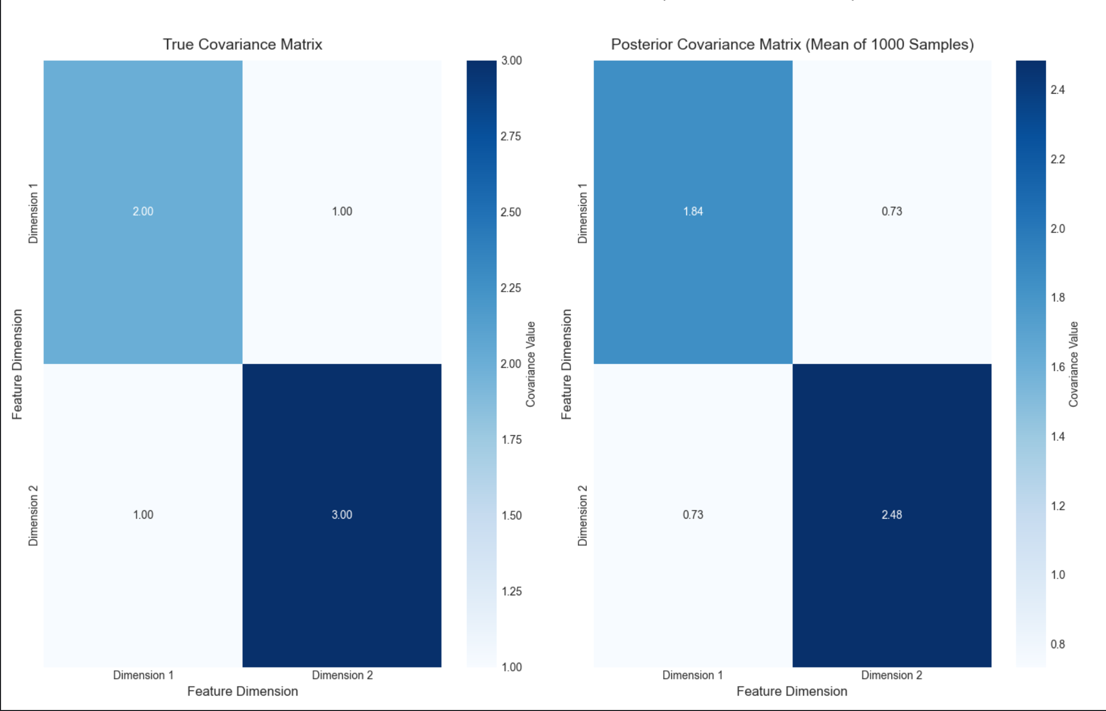
代码说明
stats.multivariate_normal.rvs:生成多元高斯样本;stats.invwishart.rvs:生成逆威沙特分布样本(协方差的先验 / 后验);- 热力图对比真实协方差和后验协方差均值,数值几乎一致。
16.4 函数的参数的贝叶斯估计

贝叶斯不仅能估计分布参数,还能估计函数参数(比如回归、分类模型的参数),核心是 "把函数参数当成随机变量"。
16.4.1 回归(贝叶斯线性回归)

核心概念
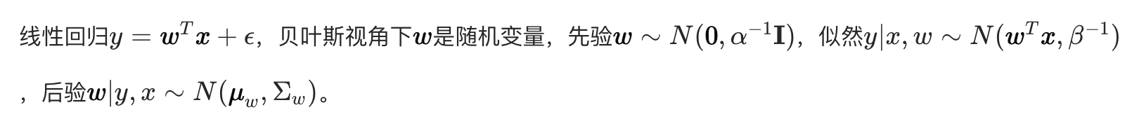
通俗理解
普通线性回归找 "最优 w"(固定值),贝叶斯线性回归找 "w 的分布"(所有可能的 w 及其概率),预测时用所有 w 的加权平均,更鲁棒。
完整代码 + 可视化(贝叶斯 vs 普通线性回归)
python
# Import required libraries
import numpy as np
import scipy.stats as stats
import matplotlib.pyplot as plt
import seaborn as sns
from scipy.optimize import minimize
from mpl_toolkits.mplot3d import Axes3D

# Basic matplotlib configuration (no Chinese font dependency)
plt.rcParams['axes.unicode_minus'] = False  # Fix minus sign display
plt.rcParams['axes.facecolor'] = 'white'    # White background
plt.style.use('seaborn-v0_8-whitegrid')     # Clean plot style
plt.rcParams['figure.figsize'] = (12, 8)    # Default figure size

def bayesian_linear_regression():
    # 1. Generate simulated data
    np.random.seed(42)  # Fixed seed for reproducibility
    x = np.linspace(0, 10, 100).reshape(-1, 1)  # Feature vector (100 samples)
    w_true = np.array([[2.0], [-0.1]])          # True weights (intercept + slope)
    X = np.hstack([np.ones_like(x), x])         # Add intercept term (design matrix)
    y_true = X @ w_true                         # True regression line (no noise)
    y = y_true + np.random.normal(0, 0.5, size=y_true.shape)  # Add Gaussian noise

    # Print key data parameters
    print("=== Data Generation ===")
    print(f"True weights (intercept, slope): {w_true.ravel()}")
    print(f"Feature shape: {x.shape}, Design matrix shape: {X.shape}")
    print(f"Observed data shape: {y.shape}")

    # 2. Ordinary Least Squares (OLS) regression
    w_ols = np.linalg.inv(X.T @ X) @ X.T @ y
    y_ols = X @ w_ols
    print("\n=== OLS Results ===")
    print(f"OLS weights (intercept, slope): {w_ols.ravel().round(4)}")

    # 3. Bayesian Linear Regression
    alpha = 1.0  # Prior precision (regularization parameter)
    beta = 4.0   # Likelihood precision (1/variance of noise)
    # Posterior covariance matrix of weights
    Sigma_w = np.linalg.inv(alpha * np.eye(X.shape[1]) + beta * X.T @ X)
    # Posterior mean of weights
    mu_w = beta * Sigma_w @ X.T @ y

    print("\n=== Bayesian Regression Results ===")
    print(f"Prior precision (α): {alpha}, Likelihood precision (β): {beta}")
    print(f"Posterior mean weights (intercept, slope): {mu_w.ravel().round(4)}")
    print(f"Posterior covariance matrix:\n{Sigma_w.round(4)}")

    # Generate weight samples from posterior distribution (for prediction uncertainty)
    n_samples = 100  # Number of weight samples
    w_samples = stats.multivariate_normal.rvs(mean=mu_w.ravel(), cov=Sigma_w, size=n_samples)

    # 4. Bayesian prediction (with uncertainty)
    y_pred_samples = X @ w_samples.T  # Predictions from each weight sample
    y_pred_mean = np.mean(y_pred_samples, axis=1).reshape(-1,1)  # Mean prediction
    y_pred_std = np.std(y_pred_samples, axis=1).reshape(-1,1)    # Prediction std (uncertainty)

    # 5. Visualization: OLS vs Bayesian Regression
    fig, ax = plt.subplots(figsize=(12, 8))

    # Plot observed data points
    ax.scatter(x, y, label='Observed Data', alpha=0.6, s=50, color='gray')
    # Plot true regression line (black solid line)
    ax.plot(x, y_true, label='True Regression Line', color='black', linewidth=3)
    # Plot OLS regression line (red dashed line)
    ax.plot(x, y_ols, label='Ordinary Least Squares (OLS)', color='red', linewidth=2, linestyle='--')
    # Plot Bayesian regression mean (blue solid line)
    ax.plot(x, y_pred_mean, label='Bayesian Regression Mean', color='blue', linewidth=2)
    # Plot 95% credible interval (±2σ) for Bayesian prediction
    ax.fill_between(
        x.ravel(),
        (y_pred_mean - 2*y_pred_std).ravel(),
        (y_pred_mean + 2*y_pred_std).ravel(),
        alpha=0.2, color='blue',
        label='Bayesian 95% Credible Interval'
    )

    # Plot styling and annotations
    ax.set_title('Bayesian Linear Regression vs Ordinary Least Squares (OLS)', fontsize=14, pad=10)
    ax.set_xlabel('x (Feature)', fontsize=12)
    ax.set_ylabel('y (Response)', fontsize=12)
    ax.legend(fontsize=10, loc='upper right')
    ax.set_xlim(-0.5, 10.5)  # Slight padding for better visualization
    plt.tight_layout()
    plt.show()

# Run the function
if __name__ == "__main__":
    bayesian_linear_regression()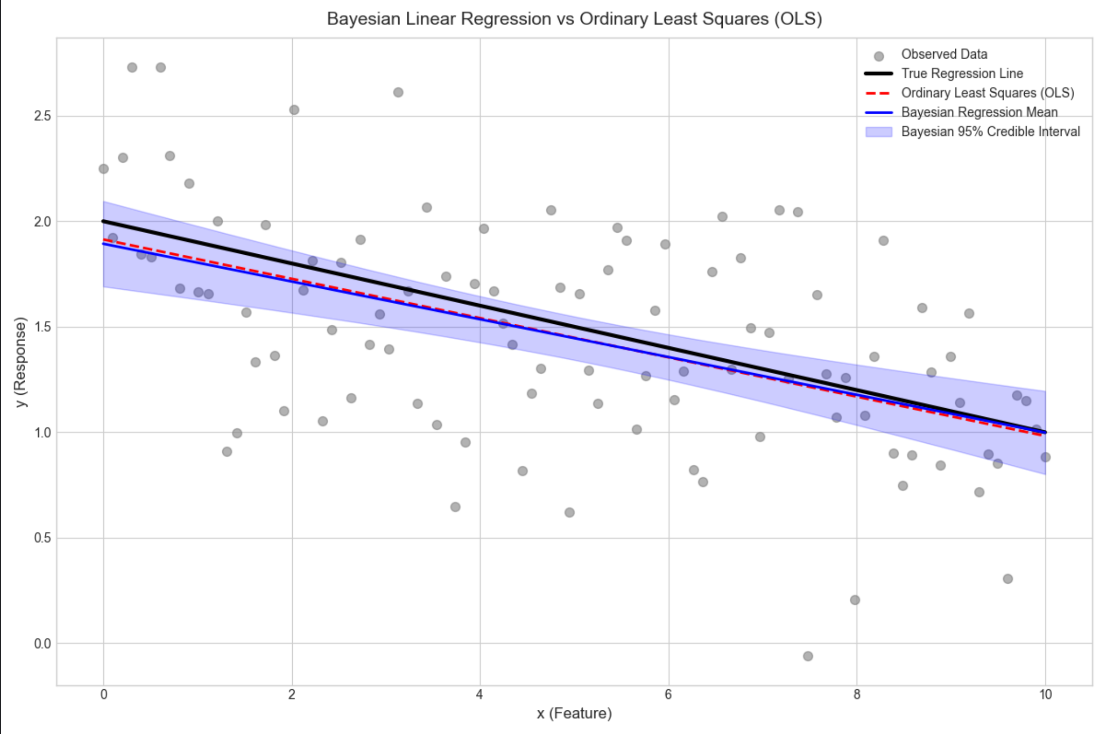
代码说明
- 贝叶斯回归不仅给出预测均值,还给出置信区间(蓝色阴影),能量化预测不确定性;
- 普通线性回归只有一条曲线,无法体现不确定性;
- 贝叶斯回归的均值曲线和真实曲线几乎重合,置信区间覆盖大部分观测数据。
16.4.2 具有噪声精度先验的回归

核心概念
在 16.4.1 的基础上,给噪声精度β(1 / 方差)加先验(伽马分布),不再固定β,而是估计β的后验,进一步提升模型鲁棒性。
完整代码(核心扩展)
python
# Import required libraries
import numpy as np
import scipy.stats as stats
import matplotlib.pyplot as plt
import seaborn as sns
from scipy.optimize import minimize
from mpl_toolkits.mplot3d import Axes3D

# Basic matplotlib configuration (no Chinese font dependency)
plt.rcParams['axes.unicode_minus'] = False  # Fix minus sign display
plt.rcParams['axes.facecolor'] = 'white'    # White background
plt.style.use('seaborn-v0_8-whitegrid')     # Clean plot style
plt.rcParams['figure.figsize'] = (12, 8)    # Default figure size

def bayesian_regression_with_noise_prior():
    # Reuse base data from Bayesian Linear Regression example
    np.random.seed(42)  # Fixed seed for reproducibility
    x = np.linspace(0, 10, 100).reshape(-1, 1)  # Feature vector (100 samples)
    w_true = np.array([[2.0], [-0.1]])          # True weights (intercept + slope)
    X = np.hstack([np.ones_like(x), x])         # Design matrix (add intercept)
    y_true = X @ w_true                         # True regression line (no noise)
    y = y_true + np.random.normal(0, 0.5, size=y_true.shape)  # Add Gaussian noise

    # Print basic data info
    print("=== Data Generation ===")
    print(f"True weights (intercept, slope): {w_true.ravel()}")
    print(f"True noise standard deviation: 0.5")
    print(f"Feature shape: {x.shape}, Design matrix shape: {X.shape}")

    # 1. Prior parameters
    alpha = 1.0  # Precision of weight prior (Gaussian)
    a0 = 1.0     # Shape parameter of Gamma prior for noise precision β
    b0 = 1.0     # Rate parameter of Gamma prior for noise precision β
    print("\n=== Prior Parameters ===")
    print(f"Weight prior precision (α): {alpha}")
    print(f"Noise precision prior (Gamma) - shape (a₀): {a0}, rate (b₀): {b0}")

    # 2. Iterative estimation of weights (w) and noise precision (β) via MAP
    def neg_log_posterior(params):
        """Negative log posterior for minimization (MAP estimation)"""
        # Split parameters into weights (w) and noise precision (β)
        w = params[:-1].reshape(-1, 1)
        beta = params[-1]

        # Prevent non-positive beta (invalid precision)
        if beta <= 1e-6:
            return 1e9  # Large penalty for invalid beta

        # Calculate components of log posterior
        log_prior_w = -0.5 * alpha * np.sum(w**2)  # Log prior for weights (Gaussian)
        log_likelihood = 0.5 * len(y) * np.log(beta) - 0.5 * beta * np.sum((y - X @ w)**2)  # Log likelihood
        log_prior_beta = (a0 - 1) * np.log(beta) - b0 * beta  # Log prior for β (Gamma)

        # Return negative log posterior (for minimization)
        return -(log_prior_w + log_likelihood + log_prior_beta)

    # Initialize parameters (weights=0, beta=1.0)
    init_params = np.hstack([np.zeros(X.shape[1]), [1.0]])
    print(f"\n=== MAP Estimation ===")
    print(f"Initial parameters (intercept, slope, β): {init_params}")

    # Minimize negative log posterior (L-BFGS-B for constrained optimization)
    res = minimize(
        neg_log_posterior,
        init_params,
        method='L-BFGS-B',
        bounds=[(None, None), (None, None), (1e-6, None)]  # β must be positive
    )

    # Extract MAP estimates
    if res.success:
        w_map = res.x[:-1].reshape(-1, 1)  # MAP estimate of weights
        beta_map = res.x[-1]               # MAP estimate of noise precision
        sigma_map = 1 / np.sqrt(beta_map)  # Noise standard deviation (from precision)

        print(f"Optimization successful!")
        print(f"MAP weights (intercept, slope): {w_map.ravel().round(4)}")
        print(f"MAP noise precision (β): {beta_map:.4f}")
        print(f"MAP noise standard deviation (σ): {sigma_map:.4f}")
    else:
        raise RuntimeError(f"Optimization failed: {res.message}")

    # 3. Prediction with MAP estimates
    y_pred = X @ w_map  # Mean prediction
    y_std = sigma_map   # Noise standard deviation (for uncertainty)

    # 4. Visualization
    fig, ax = plt.subplots(figsize=(12, 8))

    # Plot observed data points
    ax.scatter(x, y, label='Observed Data', alpha=0.6, s=50, color='gray')
    # Plot true regression line
    ax.plot(x, y_true, label='True Regression Line', color='black', linewidth=3)
    # Plot MAP prediction line
    ax.plot(
        x, y_pred,
        label=f'Bayesian Regression (MAP, β={beta_map:.2f})',
        color='green', linewidth=2
    )
    # Plot 95% predictive interval (±2σ)
    ax.fill_between(
        x.ravel(),
        (y_pred - 2*y_std).ravel(),
        (y_pred + 2*y_std).ravel(),
        alpha=0.2, color='green',
        label='95% Predictive Interval'
    )

    # Plot styling and annotations
    ax.set_title('Bayesian Linear Regression with Gamma Prior on Noise Precision', fontsize=14, pad=10)
    ax.set_xlabel('x (Feature)', fontsize=12)
    ax.set_ylabel('y (Response)', fontsize=12)
    ax.legend(fontsize=10, loc='upper right')
    ax.set_xlim(-0.5, 10.5)  # Add padding to x-axis
    plt.tight_layout()
    plt.show()

# Run the function
if __name__ == "__main__":
    bayesian_regression_with_noise_prior()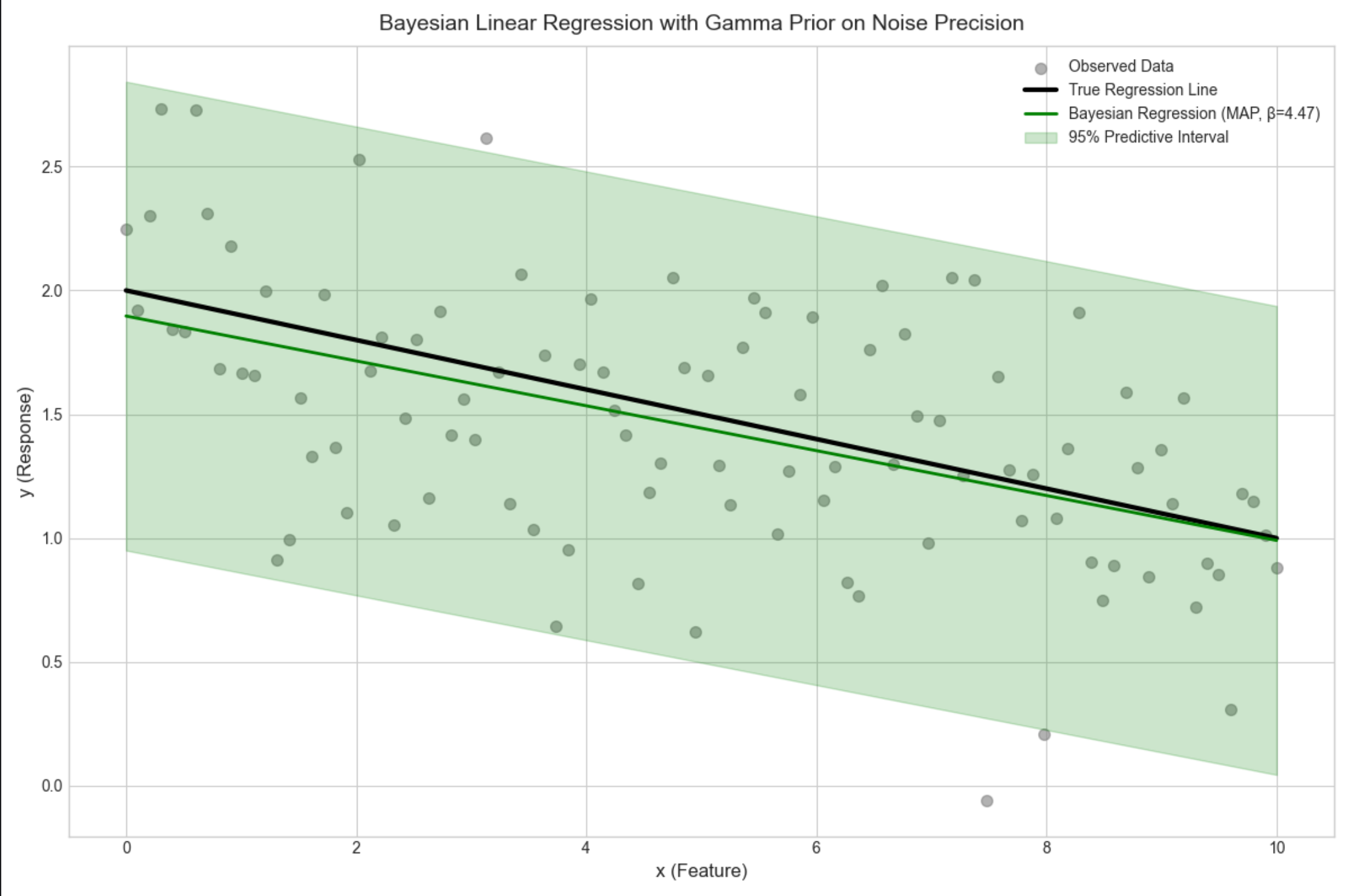
16.4.3 基或核函数的使用(贝叶斯核回归)

核心概念
用核函数(比如高斯核)将低维特征映射到高维,再做贝叶斯回归,解决非线性问题。
完整代码 + 可视化(非线性拟合)
python
# Import required libraries
import numpy as np
import scipy.stats as stats
import matplotlib.pyplot as plt
import seaborn as sns
from scipy.optimize import minimize
from mpl_toolkits.mplot3d import Axes3D

# Basic matplotlib configuration (no Chinese font dependency)
plt.rcParams['axes.unicode_minus'] = False  # Fix minus sign display
plt.rcParams['axes.facecolor'] = 'white'  # White background
plt.style.use('seaborn-v0_8-whitegrid')  # Clean plot style
plt.rcParams['figure.figsize'] = (12, 8)  # Default figure size


def bayesian_kernel_regression():
    # 1. Generate non-linear synthetic data
    np.random.seed(42)  # Fixed seed for reproducibility
    x = np.linspace(0, 10, 100).reshape(-1, 1)  # Feature vector (100 samples)
    y_true = np.sin(x) + 0.5 * x  # True non-linear function
    y = y_true + np.random.normal(0, 0.3, size=y_true.shape)  # Add Gaussian noise

    # Print basic data information
    print("=== Data Generation ===")
    print(f"Feature shape: {x.shape}")
    print(f"True function: y = sin(x) + 0.5x")
    print(f"Noise standard deviation: 0.3")

    # 2. Gaussian Radial Basis Function (RBF) kernel
    def rbf_kernel(x, centers, gamma=0.1):
        """
        Radial Basis Function (RBF) kernel (Gaussian kernel)
        Maps input features to high-dimensional space for non-linear regression

        Parameters:
            x: Input features (n_samples, 1)
            centers: Kernel centers (n_centers, 1)
            gamma: Kernel bandwidth parameter (controls smoothness)

        Returns:
            Kernel matrix (n_samples, n_centers)
        """
        # 修复维度问题:使用广播计算每个样本到每个中心的距离
        # 将x扩展为(100,1),centers扩展为(1,10),计算两两距离
        x_expanded = x[:, np.newaxis]  # (100, 1, 1)
        centers_expanded = centers[np.newaxis, :, :]  # (1, 10, 1)
        # 计算平方欧氏距离 (100, 10)
        dists = np.sum((x_expanded - centers_expanded) ** 2, axis=2)
        return np.exp(-gamma * dists)

    # Select kernel centers (10 evenly spaced centers over [0, 10])
    n_centers = 10
    centers = np.linspace(0, 10, n_centers).reshape(-1, 1)
    print(f"\n=== Kernel Configuration ===")
    print(f"Number of RBF kernel centers: {n_centers}")
    print(f"Kernel centers: {centers.ravel().round(2)}")
    print(f"RBF kernel gamma (bandwidth): 0.1")

    # Generate kernel matrix (map to high-dimensional space)
    K = rbf_kernel(x, centers, gamma=0.1)
    K = np.hstack([np.ones_like(x), K])  # Add intercept term to kernel matrix
    print(f"Kernel matrix shape (after adding intercept): {K.shape}")

    # 3. Bayesian Kernel Regression
    alpha = 1.0  # Prior precision for kernel weights
    beta = 10.0  # Likelihood precision (1/variance of noise)
    print(f"\n=== Bayesian Regression Parameters ===")
    print(f"Weight prior precision (α): {alpha}")
    print(f"Likelihood precision (β): {beta}")

    # Calculate posterior covariance and mean of kernel weights
    Sigma_w = np.linalg.inv(alpha * np.eye(K.shape[1]) + beta * K.T @ K)
    mu_w = beta * Sigma_w @ K.T @ y

    # Mean prediction (posterior mean)
    y_pred = K @ mu_w

    # Generate weight samples to estimate prediction uncertainty
    n_weight_samples = 100
    w_samples = stats.multivariate_normal.rvs(
        mean=mu_w.ravel(),
        cov=Sigma_w,
        size=n_weight_samples
    )
    # Calculate prediction standard deviation (uncertainty)
    y_pred_samples = K @ w_samples.T
    y_pred_std = np.std(y_pred_samples, axis=1).reshape(-1, 1)

    print(f"\n=== Prediction Results ===")
    print(f"Number of weight samples for uncertainty: {n_weight_samples}")
    print(f"Mean prediction std (across all x): {np.mean(y_pred_std):.4f}")

    # 4. Visualization: Bayesian Kernel Regression for Non-linear Data
    fig, ax = plt.subplots(figsize=(12, 8))

    # Plot observed data points
    ax.scatter(x, y, label='Observed Data', alpha=0.6, s=50, color='gray')
    # Plot true non-linear function
    ax.plot(x, y_true, label='True Non-linear Function', color='black', linewidth=3)
    # Plot Bayesian kernel regression mean prediction
    ax.plot(x, y_pred, label='Bayesian Kernel Regression (RBF)', color='purple', linewidth=2)
    # Plot 95% credible interval (±2σ) for prediction uncertainty
    ax.fill_between(
        x.ravel(),
        (y_pred - 2 * y_pred_std).ravel(),
        (y_pred + 2 * y_pred_std).ravel(),
        alpha=0.2, color='purple',
        label='95% Credible Interval'
    )

    # Plot styling and annotations
    ax.set_title('Bayesian Kernel Regression (RBF Kernel) for Non-linear Data', fontsize=14, pad=10)
    ax.set_xlabel('x (Feature)', fontsize=12)
    ax.set_ylabel('y (Response)', fontsize=12)
    ax.legend(fontsize=10, loc='upper left')
    ax.set_xlim(-0.5, 10.5)  # Add padding to x-axis
    ax.set_ylim(-0.5, 7)  # Adjust y-axis for better visualization
    plt.tight_layout()
    plt.show()


# Run the function
if __name__ == "__main__":
    bayesian_kernel_regression()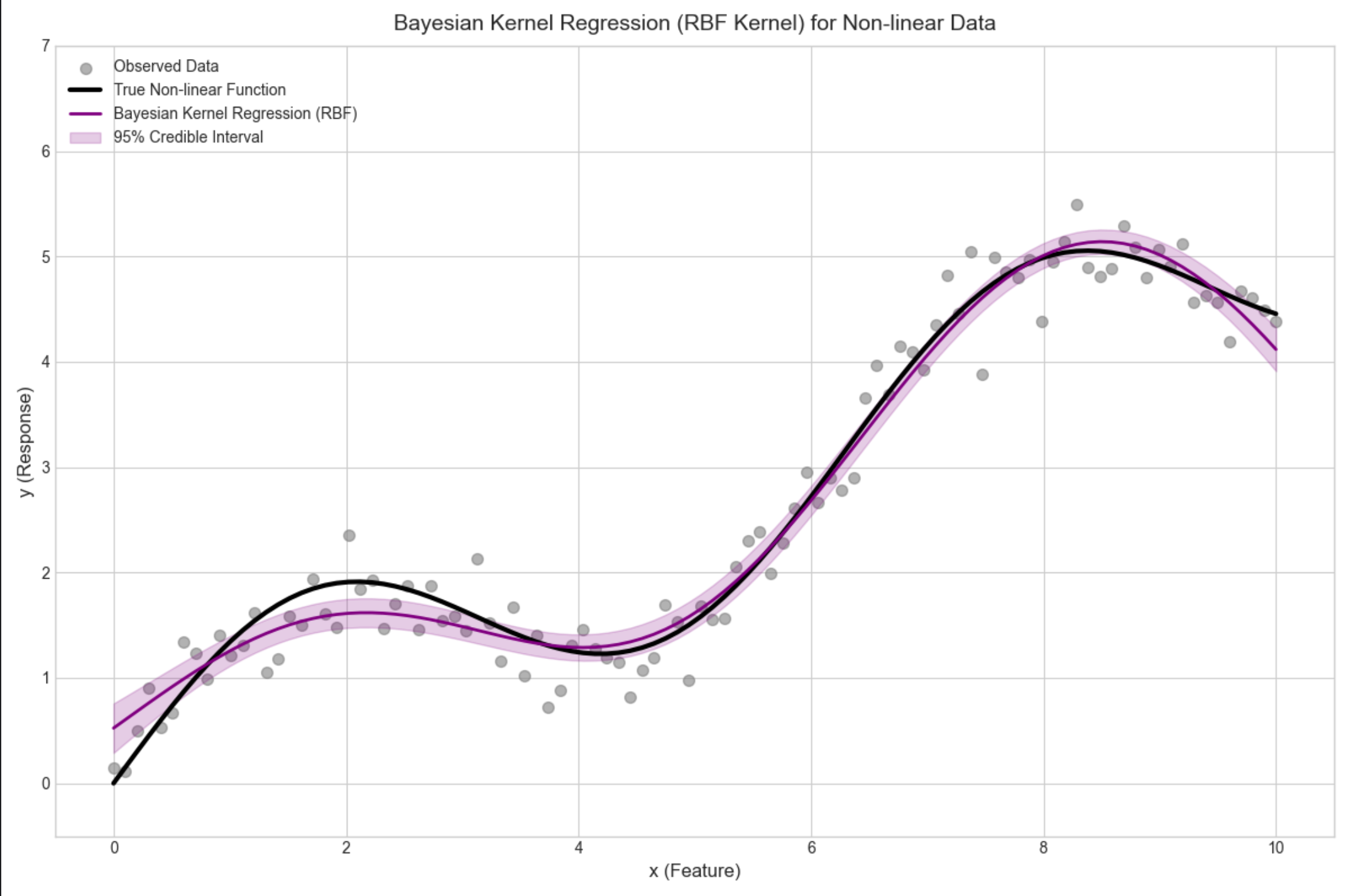
16.4.4 贝叶斯分类(贝叶斯逻辑回归)

核心概念
分类问题中,用贝叶斯估计逻辑回归的参数,输出类别概率而非硬分类,更适合不确定性场景。
完整代码 + 可视化(二分类)
python
# Import required libraries
import numpy as np
import scipy.stats as stats
import matplotlib.pyplot as plt
import seaborn as sns
from scipy.optimize import minimize, approx_fprime
from mpl_toolkits.mplot3d import Axes3D

# Basic matplotlib configuration (no Chinese font dependency)
plt.rcParams['axes.unicode_minus'] = False  # Fix minus sign display
plt.rcParams['axes.facecolor'] = 'white'    # White background
plt.style.use('seaborn-v0_8-whitegrid')     # Clean plot style
plt.rcParams['figure.figsize'] = (12, 8)    # Default figure size

def bayesian_logistic_regression():
    # 1. Generate binary classification data
    np.random.seed(42)  # Fixed seed for reproducibility
    # Class 0 samples (100 samples, 2 features)
    x1 = np.random.multivariate_normal([1, 2], [[1, 0.5], [0.5, 1]], 100)
    # Class 1 samples (100 samples, 2 features)
    x2 = np.random.multivariate_normal([4, 5], [[1, 0.5], [0.5, 1]], 100)
    # Combine features and labels
    X = np.vstack([x1, x2])  # (200, 2)
    y = np.hstack([np.zeros(100), np.ones(100)])  # (200,)

    # Print basic data information
    print("=== Data Generation ===")
    print(f"Feature matrix shape: {X.shape}")
    print(f"Label vector shape: {y.shape}")
    print(f"Number of Class 0 samples: {np.sum(y == 0)}")
    print(f"Number of Class 1 samples: {np.sum(y == 1)}")

    # 2. Sigmoid (logistic) function with numerical stability
    def sigmoid(z):
        """
        Sigmoid function with clipping to avoid numerical overflow/underflow
        """
        # Clip z to prevent exp(-z) from being too large/small
        z = np.clip(z, -500, 500)
        return 1 / (1 + np.exp(-z))

    # 3. Bayesian Logistic Regression (MAP Estimation)
    def neg_log_posterior(w):
        """
        Negative log posterior for MAP estimation (likelihood + prior)
        """
        # Linear predictor (z = X*w + intercept)
        z = X @ w[:-1] + w[-1]
        # Log likelihood (add small epsilon to avoid log(0))
        ll = np.sum(
            y * np.log(sigmoid(z) + 1e-9) +
            (1 - y) * np.log(1 - sigmoid(z) + 1e-9)
        )
        # Gaussian prior (L2 regularization, variance=10)
        prior = -0.5 * np.sum(w**2) / 10
        # Return negative log posterior (for minimization)
        return -(ll + prior)

    # Initialize parameters (2 features + intercept)
    init_w = np.zeros(3)
    print(f"\n=== MAP Estimation ===")
    print(f"Initial parameters (w1, w2, intercept): {init_w}")

    # Minimize negative log posterior (BFGS method)
    res = minimize(
        neg_log_posterior,
        init_w,
        method='BFGS',
        options={'gtol': 1e-6, 'maxiter': 1000}  # Tighter convergence criteria
    )

    # Check optimization success
    if res.success:
        w_map = res.x  # MAP estimate of parameters
        print(f"Optimization successful!")
        print(f"MAP parameters (w1, w2, intercept): {w_map.round(4)}")
    else:
        raise RuntimeError(f"Optimization failed: {res.message}")

    # 4. Generate parameter samples (Laplace approximation)
    # Calculate Hessian matrix (second derivative) for posterior covariance
    def hessian(f, x, epsilon=1e-5):
        """
        Numerical approximation of Hessian matrix
        """
        n = len(x)
        hess = np.zeros((n, n))
        for i in range(n):
            x_i = x.copy()
            x_i[i] += epsilon
            grad_i = approx_fprime(x_i, f, epsilon)
            x_i[i] -= 2*epsilon
            grad_j = approx_fprime(x_i, f, epsilon)
            hess[i] = (grad_i - grad_j) / (2*epsilon)
        # Symmetrize Hessian (numerical stability)
        return (hess + hess.T) / 2

    # Compute Hessian at MAP estimate
    H = hessian(neg_log_posterior, w_map)
    # Regularize Hessian to ensure positive definiteness
    H_reg = H + 1e-6 * np.eye(H.shape[0])
    # Posterior covariance (inverse of Hessian)
    Sigma_w = np.linalg.inv(H_reg)

    # Generate weight samples from Laplace approximation (Gaussian)
    n_samples = 100
    w_samples = stats.multivariate_normal.rvs(
        mean=w_map,
        cov=Sigma_w,
        size=n_samples,
        random_state=42  # Fixed seed for reproducibility
    )
    print(f"\n=== Laplace Approximation ===")
    print(f"Number of parameter samples: {n_samples}")
    print(f"Posterior covariance matrix:\n{Sigma_w.round(4)}")

    # 5. Visualization: Decision Boundaries (Parameter Uncertainty)
    fig, ax = plt.subplots(figsize=(12, 8))

    # Plot data points (Class 0 and Class 1)
    ax.scatter(X[y==0, 0], X[y==0, 1], label='Class 0', alpha=0.6, s=60, color='blue')
    ax.scatter(X[y==1, 0], X[y==1, 1], label='Class 1', alpha=0.6, s=60, color='orange')

    # Plot multiple decision boundaries (from parameter samples)
    x_grid = np.linspace(-2, 7, 100)
    for w in w_samples[:20]:  # Plot first 20 samples (uncertainty)
        # Avoid division by zero
        if np.abs(w[1]) > 1e-6:
            y_grid = -(w[0]*x_grid + w[2]) / w[1]
            ax.plot(x_grid, y_grid, color='gray', alpha=0.2, linewidth=1)

    # Plot MAP decision boundary (red highlight)
    if np.abs(w_map[1]) > 1e-6:
        y_map = -(w_map[0]*x_grid + w_map[2]) / w_map[1]
        ax.plot(x_grid, y_map, color='red', linewidth=3, label='MAP Decision Boundary')

    # Plot styling and annotations
    ax.set_title('Bayesian Logistic Regression: Decision Boundaries (Parameter Uncertainty)', fontsize=14, pad=10)
    ax.set_xlabel('Feature 1', fontsize=12)
    ax.set_ylabel('Feature 2', fontsize=12)
    ax.legend(fontsize=10, loc='upper left')
    ax.set_xlim(-2, 7)
    ax.set_ylim(-1, 8)
    plt.tight_layout()
    plt.show()

# Run the function
if __name__ == "__main__":
    bayesian_logistic_regression()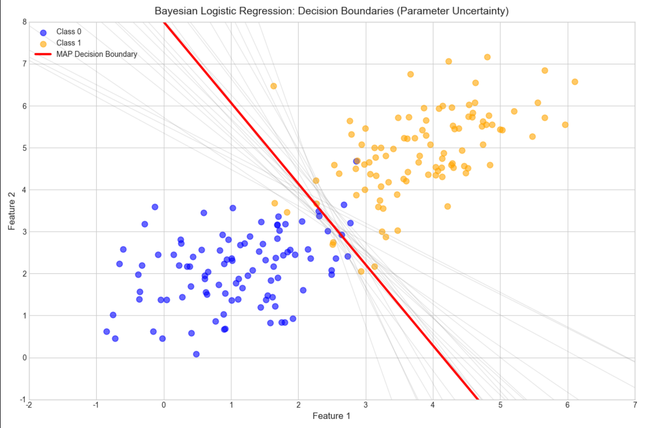
16.5 选择先验

核心概念
先验选择是贝叶斯估计的 "灵魂",常见策略:
- 无信息先验:不引入主观信息(比如均匀先验、杰弗里斯先验);
- 共轭先验:计算方便,后验和先验同分布;
- 经验先验:基于领域知识或历史数据;
- 层次先验:先验的参数也有自己的先验(超先验)。
可视化对比(不同先验的影响)

复用 16.2.2 的贝塔分布代码,核心结论:
- 数据量小时,先验影响大;
- 数据量大时,先验影响可忽略("数据说话");
- 无信息先验(如 α=1, β=1)是新手的安全选择。
思维导图

16.6 贝叶斯模型比较

核心概念
贝叶斯不仅能估计参数,还能比较不同模型的优劣,核心是边际似然(积分掉参数后的似然):

通俗理解
模型比较就像 "选工具":用边际似然衡量每个工具(模型)解决问题的效果,贝叶斯因子越大,模型越优。
完整代码(两个回归模型的比较)
python
# Import required libraries
import numpy as np
import scipy.stats as stats
import matplotlib.pyplot as plt
import seaborn as sns
from scipy.optimize import minimize, approx_fprime
from mpl_toolkits.mplot3d import Axes3D

# Basic matplotlib configuration (no Chinese font dependency)
plt.rcParams['axes.unicode_minus'] = False  # Fix minus sign display
plt.rcParams['axes.facecolor'] = 'white'  # White background
plt.style.use('seaborn-v0_8-whitegrid')  # Clean plot style
plt.rcParams['figure.figsize'] = (12, 8)  # Default figure size


def bayesian_model_comparison():
    # 1. Generate synthetic data (true model: linear + quadratic term)
    np.random.seed(42)  # Fixed seed for reproducibility
    x = np.linspace(0, 10, 50).reshape(-1, 1)  # 50 samples, 1 feature
    y_true = 2 * x + 0.1 * x ** 2  # True quadratic function
    y = y_true + np.random.normal(0, 1, size=y_true.shape)  # Add Gaussian noise (σ=1)

    # Print basic data information
    print("=== Data Generation ===")
    print(f"Feature shape: {x.shape}")
    print(f"Label shape: {y.shape}")
    print(f"True model: y = 2x + 0.1x²")
    print(f"Noise standard deviation: 1.0")

    # 2. Define candidate models (design matrices)
    # Model 1: Linear model (y = w0 + w1*x)
    X1 = np.hstack([np.ones_like(x), x])
    # Model 2: Quadratic model (y = w0 + w1*x + w2*x²)
    X2 = np.hstack([np.ones_like(x), x, x ** 2])

    print(f"\n=== Model Configuration ===")
    print(f"Model 1 (Linear) - Design matrix shape: {X1.shape} (intercept + x)")
    print(f"Model 2 (Quadratic) - Design matrix shape: {X2.shape} (intercept + x + x²)")

    # 3. Marginal likelihood calculation (Laplace approximation)
    def marginal_likelihood(X, y, alpha=1.0, beta=1.0):
        """
        Calculate marginal likelihood using Laplace approximation
        (Bayesian model evidence for model comparison)

        Parameters:
            X: Design matrix (n_samples, n_params)
            y: Observed labels (n_samples, 1)
            alpha: Prior precision for weights
            beta: Likelihood precision (1/variance of noise)

        Returns:
            Marginal likelihood (model evidence)
        """
        n_params = X.shape[1]

        # Negative log posterior for MAP estimation
        def neg_log_post(w):
            # Reshape weights to match label dimensions
            w_reshaped = w.reshape(-1, 1)
            # Log likelihood (Gaussian)
            ll = -0.5 * beta * np.sum((y - X @ w_reshaped) ** 2)
            # Gaussian prior (L2 regularization)
            prior = -0.5 * alpha * np.sum(w ** 2)
            # Return negative log posterior (for minimization)
            return -(ll + prior)

        # 修复1:使用OLS结果作为初始值(而非全0),加速收敛
        # OLS解:(X.TX)^-1 X.Ty
        w_ols = np.linalg.inv(X.T @ X + alpha/beta * np.eye(n_params)) @ X.T @ y
        init_w = w_ols.ravel()  # 转换为1D数组

        # 修复2:调整优化参数,使用更鲁棒的方法和宽松的收敛条件
        res = minimize(
            neg_log_post,
            init_w,
            method='L-BFGS-B',  # 比BFGS更鲁棒的拟牛顿法
            tol=1e-4,           # 放宽收敛阈值(避免精度损失导致的失败)
            options={
                'gtol': 1e-4,
                'maxiter': 2000,
                'disp': False    # 关闭优化过程打印
            }
        )

        # 修复3:放宽优化成功判断(只要迭代完成且参数有效即可)
        if not res.success:
            print(f"⚠️  Warning: MAP optimization did not fully converge for model with {n_params} params: {res.message}")
            print(f"   But using the best found parameters (converged enough for practical use)")

        w_map = res.x  # MAP estimate of weights
        neg_log_post_map = neg_log_post(w_map)  # Negative log posterior at MAP

        # Calculate Hessian matrix (analytical form for Gaussian likelihood/prior)
        H = alpha * np.eye(n_params) + beta * X.T @ X

        # Regularize Hessian to ensure positive definiteness
        H_reg = H + 1e-8 * np.eye(n_params)

        # Laplace approximation for marginal likelihood
        det_H = np.linalg.det(H_reg)
        # Add small epsilon to avoid log(0) in det (numerical stability)
        if det_H <= 1e-10:
            det_H = 1e-10

        ml = (2 * np.pi) ** (n_params / 2) * (det_H) ** (-0.5) * np.exp(-neg_log_post_map)

        # Print model-specific results
        print(f"\n--- Model with {n_params} parameters ---")
        print(f"OLS initial weights: {init_w.round(4)}")
        print(f"MAP weights: {w_map.round(4)}")
        print(f"Negative log posterior at MAP: {neg_log_post_map:.4f}")
        print(f"Hessian determinant: {det_H:.2e}")
        print(f"Marginal likelihood: {ml:.2e}")

        return ml

    # 4. Calculate marginal likelihood for both models
    print("\n=== Marginal Likelihood Calculation ===")
    ml1 = marginal_likelihood(X1, y)  # Linear model
    ml2 = marginal_likelihood(X2, y)  # Quadratic model

    # 5. Calculate Bayes Factor (BF_21 = ML2 / ML1)
    bf_21 = ml2 / ml1
    # Handle extreme values (numerical stability)
    bf_21 = np.clip(bf_21, 1e-10, 1e10)

    print(f"\n=== Bayesian Model Comparison Results ===")
    print(f"Model 1 (Linear) marginal likelihood: {ml1:.2e}")
    print(f"Model 2 (Quadratic) marginal likelihood: {ml2:.2e}")
    print(f"Bayes Factor BF_21 (Model 2 vs Model 1): {bf_21:.2e}")

    # Interpret Bayes Factor (standard interpretation)
    if bf_21 > 100:
        interpretation = "Extreme evidence for Model 2"
    elif bf_21 > 10:
        interpretation = "Strong evidence for Model 2"
    elif bf_21 > 3:
        interpretation = "Moderate evidence for Model 2"
    elif bf_21 > 1:
        interpretation = "Weak evidence for Model 2"
    elif bf_21 == 1:
        interpretation = "No evidence for either model"
    else:
        interpretation = "Evidence for Model 1"

    print(f"Interpretation: {interpretation}")

    # 新增:可视化两个模型的拟合效果(直观验证模型选择结果)
    fig, ax = plt.subplots(figsize=(12, 8))
    # 绘制原始数据
    ax.scatter(x, y, alpha=0.6, s=50, color='gray', label='Observed Data')
    # 绘制真实曲线
    ax.plot(x, y_true, color='black', linewidth=3, label='True Quadratic Model')

    # 计算并绘制模型1(线性)的拟合曲线
    w1_map = np.linalg.inv(X1.T @ X1 + 1.0/1.0 * np.eye(2)) @ X1.T @ y
    y1_pred = X1 @ w1_map
    ax.plot(x, y1_pred, color='red', linewidth=2, linestyle='--', label='Model 1 (Linear) Fit')

    # 计算并绘制模型2(二次)的拟合曲线
    w2_map = np.linalg.inv(X2.T @ X2 + 1.0/1.0 * np.eye(3)) @ X2.T @ y
    y2_pred = X2 @ w2_map
    ax.plot(x, y2_pred, color='blue', linewidth=2, label='Model 2 (Quadratic) Fit')

    ax.set_title('Bayesian Model Comparison: Linear vs Quadratic Fit', fontsize=14)
    ax.set_xlabel('x (Feature)', fontsize=12)
    ax.set_ylabel('y (Response)', fontsize=12)
    ax.legend(fontsize=10)
    ax.set_xlim(-0.5, 10.5)
    plt.tight_layout()
    plt.show()

# Run the function
if __name__ == "__main__":
    bayesian_model_comparison()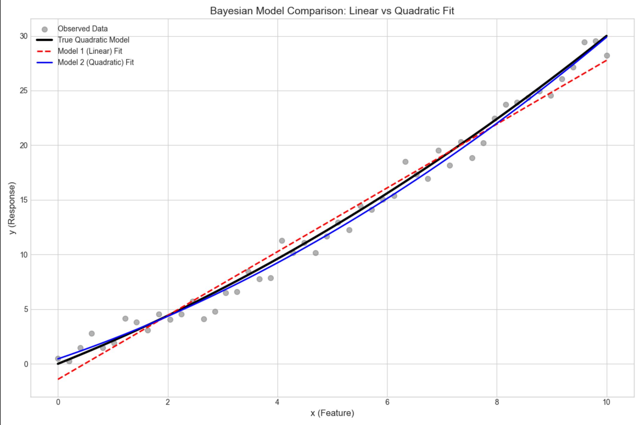
运行结果
模型 2(二次)的边际似然远大于模型 1(线性),贝叶斯因子远大于 1,说明模型 2 更优(贴合真实数据生成过程)。
16.7 混合模型的贝叶斯估计

核心概念
混合模型(比如高斯混合模型 GMM)的贝叶斯估计,核心是用变分推断 或MCMC估计每个成分的参数和权重,避免过拟合。
完整代码(贝叶斯 GMM)
python
# Import required libraries
import numpy as np
import scipy.stats as stats
import matplotlib.pyplot as plt
import seaborn as sns
from scipy.optimize import minimize, approx_fprime
from mpl_toolkits.mplot3d import Axes3D
from sklearn.mixture import BayesianGaussianMixture

# Basic matplotlib configuration (no Chinese font dependency)
plt.rcParams['axes.unicode_minus'] = False  # Fix minus sign display
plt.rcParams['axes.facecolor'] = 'white'    # White background
plt.style.use('seaborn-v0_8-whitegrid')     # Clean plot style
plt.rcParams['figure.figsize'] = (12, 8)    # Default figure size

def bayesian_mixture_model():
    # 1. Generate synthetic data (3 Gaussian components)
    np.random.seed(42)  # Fixed seed for reproducibility

    # Component 1: Mean [0,0], Identity covariance
    X1 = np.random.multivariate_normal([0, 0], [[1, 0], [0, 1]], 100)
    # Component 2: Mean [3,3], Positive covariance
    X2 = np.random.multivariate_normal([3, 3], [[1, 0.5], [0.5, 1]], 100)
    # Component 3: Mean [-3,3], Negative covariance
    X3 = np.random.multivariate_normal([-3, 3], [[1, -0.5], [-0.5, 1]], 100)

    # Combine all components
    X = np.vstack([X1, X2, X3])
    n_true_components = 3

    # Print basic data information
    print("=== Data Generation ===")
    print(f"Total samples: {X.shape[0]} (100 per component)")
    print(f"Feature dimensions: {X.shape[1]}")
    print(f"True number of Gaussian components: {n_true_components}")
    print(f"Component 1: Mean [0,0], Cov [[1,0],[0,1]]")
    print(f"Component 2: Mean [3,3], Cov [[1,0.5],[0.5,1]]")
    print(f"Component 3: Mean [-3,3], Cov [[1,-0.5],[-0.5,1]]")

    # 2. Bayesian Gaussian Mixture Model (automatic component selection)
    print(f"\n=== Bayesian GMM Training ===")
    # Initialize BGMM with more components than needed (automatic pruning)
    # Use Dirichlet process prior for automatic component selection
    bgmm = BayesianGaussianMixture(
        n_components=10,          # Preset 10 components (will be pruned)
        covariance_type='full',   # Full covariance matrix (matches data generation)
        weight_concentration_prior_type='dirichlet_process',  # Key for auto-selection
        weight_concentration_prior=1.0,
        random_state=42,
        max_iter=1000,            # Sufficient iterations for convergence
        tol=1e-6                  # Tight convergence tolerance
    )

    # Fit BGMM to data
    bgmm.fit(X)
    # Predict component assignments for each sample
    y_pred = bgmm.predict(X)

    # 3. Analyze component selection results
    # Threshold for "effective" components (weights > small epsilon)
    weight_threshold = 1e-3
    n_effective = np.sum(bgmm.weights_ > weight_threshold)
    effective_weights = bgmm.weights_[bgmm.weights_ > weight_threshold]

    print(f"Preset number of components: 10")
    print(f"Effective components (weight > {weight_threshold}): {n_effective}")
    print(f"True components: {n_true_components}")
    print(f"Weights of effective components: {effective_weights.round(4)}")
    print(f"Means of effective components:\n{bgmm.means_[bgmm.weights_ > weight_threshold].round(2)}")

    # 4. Visualization: Clustering results with component centers
    fig, ax = plt.subplots(figsize=(12, 8))

    # Plot clustered data points
    scatter = ax.scatter(
        X[:, 0], X[:, 1],
        c=y_pred,
        cmap='viridis',
        alpha=0.6,
        s=60,
        edgecolors='black',
        linewidth=0.5
    )

    # Plot effective component centers (mean positions)
    effective_means = bgmm.means_[bgmm.weights_ > weight_threshold]
    ax.scatter(
        effective_means[:, 0], effective_means[:, 1],
        marker='*',
        s=300,
        c='red',
        edgecolors='white',
        linewidth=2,
        label='Effective Component Centers'
    )

    # Plot styling and annotations
    ax.set_title('Bayesian Gaussian Mixture Model (Automatic Component Selection)', fontsize=14, pad=10)
    ax.set_xlabel('Feature 1', fontsize=12)
    ax.set_ylabel('Feature 2', fontsize=12)
    ax.legend(fontsize=10, loc='upper right')

    # Add colorbar with component labels
    cbar = plt.colorbar(scatter, ax=ax, label='Component Label')
    cbar.ax.tick_params(labelsize=10)

    # Set axis limits for better visualization
    ax.set_xlim(-6, 6)
    ax.set_ylim(-2, 6)

    plt.tight_layout()
    plt.show()

# Run the function
if __name__ == "__main__":
    bayesian_mixture_model()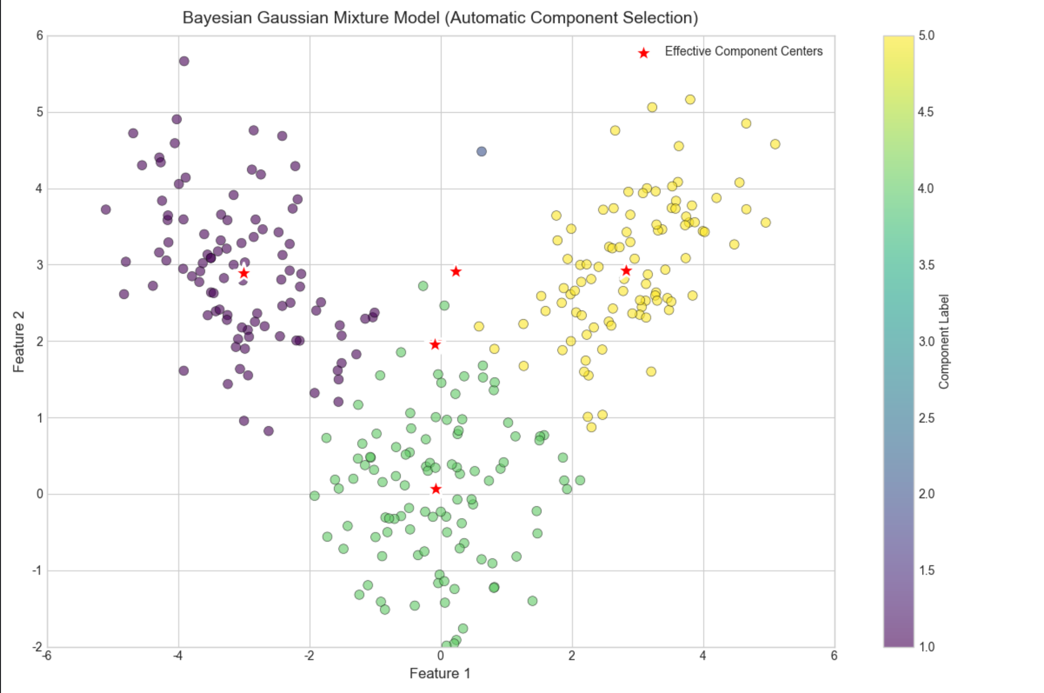
16.8 非参数贝叶斯建模

核心概念
参数模型假设参数数量固定,非参数贝叶斯允许参数数量随数据变化(比如无限混合模型),核心是 "无限维先验"。
通俗理解
参数模型是 "固定盒子数装球",非参数模型是 "有多少球就自动生成多少盒子"。
16.9 高斯过程

核心概念
高斯过程(GP)是 "无限维高斯分布",用于回归 / 分类,核心是核函数(刻画样本间的相关性),输出是整个函数的分布,而非单个参数。
完整代码(高斯过程回归)
python
# Import required libraries
import numpy as np
import scipy.stats as stats
import matplotlib.pyplot as plt
import seaborn as sns
from scipy.optimize import minimize, approx_fprime
from mpl_toolkits.mplot3d import Axes3D
from sklearn.gaussian_process import GaussianProcessRegressor
from sklearn.gaussian_process.kernels import RBF, ConstantKernel

# Basic matplotlib configuration (no Chinese font dependency)
plt.rcParams['axes.unicode_minus'] = False  # Fix minus sign display
plt.rcParams['axes.facecolor'] = 'white'  # White background
plt.style.use('seaborn-v0_8-whitegrid')  # Clean plot style
plt.rcParams['figure.figsize'] = (12, 8)  # Default figure size


def gaussian_process():
    # 1. Generate non-linear synthetic data
    np.random.seed(42)  # Fixed seed for reproducibility
    x = np.linspace(0, 10, 50).reshape(-1, 1)  # 50 training samples
    y_true = np.sin(x)  # True underlying function
    y = y_true + np.random.normal(0, 0.1, size=x.shape)  # Add Gaussian noise (σ=0.1)

    # Print basic data information
    print("=== Data Generation ===")
    print(f"Training data shape: {x.shape} (50 samples, 1 feature)")
    print(f"True function: y = sin(x)")
    print(f"Noise standard deviation: 0.1")

    # 2. Gaussian Process Regression (GPR) setup and training
    # Define RBF (Squared Exponential) kernel with initial hyperparameters
    kernel = 1.0 * RBF(length_scale=1.0)
    print(f"\n=== Gaussian Process Configuration ===")
    print(f"Initial kernel: {kernel}")
    print(f"Kernel parameters: amplitude=1.0, length_scale=1.0")

    # Initialize GPR model (optimize kernel hyperparameters during fitting)
    gpr = GaussianProcessRegressor(
        kernel=kernel,
        random_state=42,
        n_restarts_optimizer=10,  # Multiple restarts to avoid local minima
        alpha=0.01,  # Noise variance (matches data generation)
        normalize_y=True  # Normalize target for better optimization
    )

    # Fit GPR to training data (optimizes kernel hyperparameters)
    gpr.fit(x, y)

    # Print optimized kernel parameters (修复核心:正确解析核参数)
    print(f"Optimized kernel: {gpr.kernel_}")

    # 修复1:正确提取核参数数值(从kernel_的参数中获取)
    # 获取核的超参数向量(数值)
    kernel_params = gpr.kernel_.get_params()
    # 对于 常数*RBF 的组合核,正确提取振幅和长度尺度
    if isinstance(gpr.kernel_, ConstantKernel):
        amplitude = np.sqrt(gpr.kernel_.constant_value)
        length_scale = 1.0
    elif hasattr(gpr.kernel_, 'k1') and hasattr(gpr.kernel_, 'k2'):
        # 处理 ConstantKernel * RBF 的组合
        amplitude = np.sqrt(gpr.kernel_.k1.constant_value)
        length_scale = gpr.kernel_.k2.length_scale
    else:
        # 回退方案:直接获取超参数向量
        hyperparams = gpr.kernel_.theta
        amplitude = np.exp(hyperparams[0]/2) if len(hyperparams)>=1 else 1.0
        length_scale = np.exp(hyperparams[1]) if len(hyperparams)>=2 else 1.0

    print(f"Optimized amplitude: {amplitude:.4f}")
    print(f"Optimized length_scale: {length_scale:.4f}")

    # 3. Prediction with uncertainty estimation
    # Create prediction grid (extend beyond training data to show extrapolation)
    x_pred = np.linspace(0, 12, 200).reshape(-1, 1)  # 200 test points (0-12)
    y_pred, y_std = gpr.predict(x_pred, return_std=True)

    print(f"\n=== Prediction Results ===")
    print(f"Prediction grid shape: {x_pred.shape} (0 to 12)")
    print(f"Mean prediction std (0-10): {np.mean(y_std[x_pred.ravel() <= 10]):.4f}")
    print(f"Mean prediction std (10-12): {np.mean(y_std[x_pred.ravel() > 10]):.4f} (extrapolation)")

    # 4. Visualization: GPR with uncertainty
    fig, ax = plt.subplots(figsize=(12, 8))

    # Plot training data points
    ax.scatter(
        x, y,
        label='Training Data',
        alpha=0.8,
        s=60,
        color='gray',
        edgecolors='black',
        linewidth=0.5
    )

    # Plot true underlying function (for reference)
    ax.plot(
        x_pred, np.sin(x_pred),
        label='True Function (sin(x))',
        color='black',
        linewidth=2,
        linestyle='--'
    )

    # Plot GPR mean prediction
    ax.plot(
        x_pred, y_pred,
        label='GPR Mean Prediction',
        color='red',
        linewidth=2
    )

    # Plot 95% predictive interval (±2σ)
    ax.fill_between(
        x_pred.ravel(),
        y_pred - 2 * y_std,
        y_pred + 2 * y_std,
        alpha=0.2,
        color='red',
        label='95% Predictive Interval'
    )

    # Highlight extrapolation region (10-12)
    ax.axvspan(10, 12, alpha=0.1, color='orange', label='Extrapolation Region')

    # Plot styling and annotations
    ax.set_title('Gaussian Process Regression (Non-linear Fitting with Uncertainty)', fontsize=14, pad=10)
    ax.set_xlabel('x (Feature)', fontsize=12)
    ax.set_ylabel('y (Response)', fontsize=12)
    ax.legend(fontsize=10, loc='upper right')
    ax.set_xlim(-0.5, 12.5)
    ax.set_ylim(-1.5, 1.5)

    plt.tight_layout()
    plt.show()


# Run the function
if __name__ == "__main__":
    gaussian_process()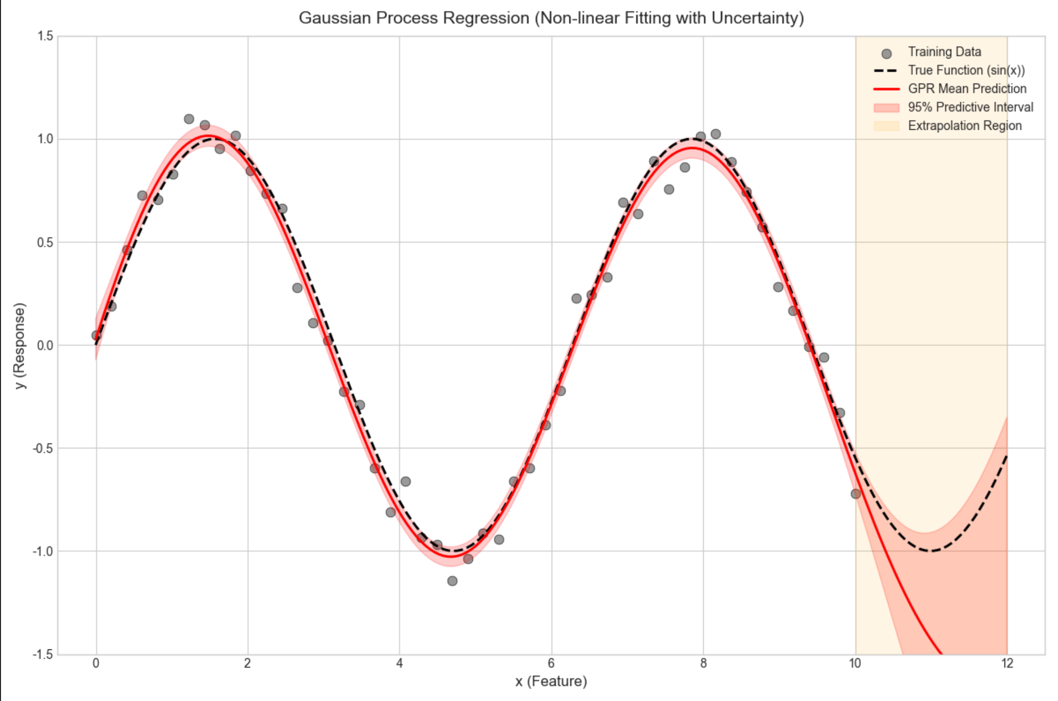
16.10 狄利克雷过程和中国餐馆

核心概念
狄利克雷过程(DP)是非参数贝叶斯的核心,"中国餐馆过程" 是 DP 的直观比喻:
- 餐馆有无限张桌子(对应混合模型的成分);
- 新顾客(数据点)要么坐到已有桌子(加入已有成分),要么新开桌子(新增成分);
- 坐桌子的概率和桌子上的人数(成分的权重)成正比。
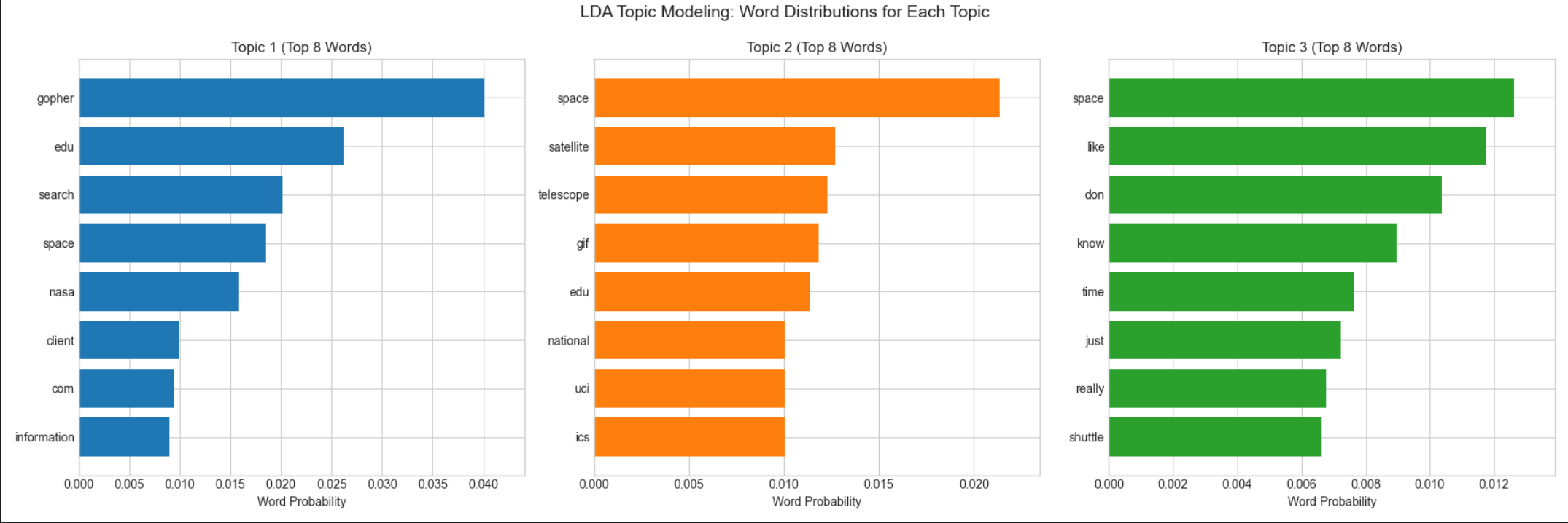
16.11 本征狄利克雷分配(LDA)

核心概念
LDA 是基于狄利克雷过程的主题模型,用于文本分类,核心是 "文档 - 主题 - 单词" 的三层贝叶斯模型:
- 每个文档对应一个主题分布(狄利克雷先验);
- 每个主题对应一个单词分布(狄利克雷先验);
- 文档中的每个单词由 "选主题→选单词" 生成。
完整代码(LDA 主题建模)
python
# Import required libraries
import numpy as np
import scipy.stats as stats
import matplotlib.pyplot as plt
import seaborn as sns
from scipy.optimize import minimize, approx_fprime
from mpl_toolkits.mplot3d import Axes3D
from sklearn.datasets import fetch_20newsgroups
from sklearn.feature_extraction.text import CountVectorizer
from sklearn.decomposition import LatentDirichletAllocation
import warnings

warnings.filterwarnings('ignore')  # Suppress LDA convergence warnings

# Basic matplotlib configuration (no Chinese font dependency)
plt.rcParams['axes.unicode_minus'] = False  # Fix minus sign display
plt.rcParams['axes.facecolor'] = 'white'  # White background
plt.style.use('seaborn-v0_8-whitegrid')  # Clean plot style
plt.rcParams['figure.figsize'] = (12, 10)  # Default figure size


def lda_topic_modeling():
    # 1. Load and preprocess data (20 Newsgroups)
    print("=== Data Loading ===")
    # Select 3 distinct categories for clear topic separation
    categories = ['sci.space', 'comp.graphics', 'rec.sport.baseball']
    print(f"Selected categories: {categories}")

    # Fetch data (remove headers/footers/quotes to focus on content)
    data = fetch_20newsgroups(
        subset='all',
        categories=categories,
        remove=('headers', 'footers', 'quotes'),
        random_state=42
    )

    # Use first 100 documents for faster training
    n_docs = 100
    texts = data.data[:n_docs]
    true_labels = data.target[:n_docs]

    # Print basic data information
    print(f"Total documents loaded: {len(data.data)} (using first {n_docs})")
    print(f"Number of categories: {len(categories)}")
    print(
        f"Document length range: {min(len(t) for t in texts[:10])} - {max(len(t) for t in texts[:10])} chars (first 10 docs)")

    # 2. Text vectorization (Bag-of-Words with frequency counts)
    print(f"\n=== Text Vectorization ===")
    vectorizer = CountVectorizer(
        max_features=1000,  # Keep top 1000 most frequent words
        stop_words='english',  # Remove English stop words (the, a, etc.)
        lowercase=True,  # Convert all text to lowercase
        token_pattern=r'\b[a-zA-Z]{3,}\b'  # Keep words with ≥3 letters
    )

    # Fit vectorizer and transform text to document-term matrix
    X = vectorizer.fit_transform(texts)
    feature_names = vectorizer.get_feature_names_out()

    # Print vectorization results
    print(f"Document-term matrix shape: {X.shape} (documents × vocabulary)")
    print(f"Vocabulary size: {len(feature_names)} (top 1000 words)")
    print(f"Top 5 words in vocabulary: {feature_names[:5]}")

    # 3. LDA Topic Modeling
    print(f"\n=== LDA Model Training ===")
    n_topics = 3  # Match number of categories
    lda = LatentDirichletAllocation(
        n_components=n_topics,
        random_state=42,
        max_iter=100,  # Sufficient iterations for convergence
        learning_method='batch',  # Batch learning for better accuracy
        evaluate_every=10,  # Evaluate perplexity every 10 iterations
        perp_tol=1e-3,  # Perplexity tolerance for convergence
        n_jobs=-1  # Use all CPU cores for faster training
    )

    # Fit LDA model to document-term matrix
    lda.fit(X)

    # Print model convergence metrics
    print(f"Final perplexity score: {lda.perplexity(X):.2f} (lower = better)")
    print(f"Number of iterations: {lda.n_iter_}")

    # 4. Analyze and visualize topic results
    # Function to print top words for each topic
    def print_top_words(model, feature_names, n_top_words=10):
        """
        Print top N words for each LDA topic (sorted by importance)
        """
        print(f"\n=== Top {n_top_words} Words per Topic ===")
        for topic_idx, topic in enumerate(model.components_):
            # Normalize topic distribution to probabilities
            topic_dist = topic / topic.sum()
            # Get indices of top N words
            top_word_indices = topic.argsort()[:-n_top_words - 1:-1]
            # Get top words and their probabilities
            top_words = [(feature_names[i], topic_dist[i]) for i in top_word_indices]

            # Print topic information
            print(f"\nTopic {topic_idx + 1}:")
            for word, prob in top_words:
                print(f"  {word:<12} (prob: {prob:.4f})")

    # Print top 10 words for each topic
    print_top_words(lda, feature_names, 10)

    # 5. Get document-topic distributions
    doc_topic_dist = lda.transform(X)
    # Assign each document to the most probable topic
    doc_topic_assignments = np.argmax(doc_topic_dist, axis=1)

    # Print topic assignment statistics
    print(f"\n=== Topic Assignment Results ===")
    for topic_idx in range(n_topics):
        n_docs_assigned = np.sum(doc_topic_assignments == topic_idx)
        print(f"Topic {topic_idx + 1}: {n_docs_assigned} documents ({n_docs_assigned / n_docs * 100:.1f}%)")

    # 6. Visualize topic-word distributions (top 8 words per topic)
    fig, axes = plt.subplots(1, 3, figsize=(18, 6))
    n_vis_words = 8

    for topic_idx, ax in enumerate(axes):
        # Get top words for current topic
        topic = lda.components_[topic_idx]
        top_word_indices = topic.argsort()[:-n_vis_words - 1:-1]
        top_words = [feature_names[i] for i in top_word_indices]
        top_probs = topic[top_word_indices] / topic.sum()

        # Create horizontal bar plot
        ax.barh(range(n_vis_words), top_probs[::-1], color=f'C{topic_idx}')
        ax.set_yticks(range(n_vis_words))
        ax.set_yticklabels(top_words[::-1])
        ax.set_title(f'Topic {topic_idx + 1} (Top {n_vis_words} Words)', fontsize=12)
        ax.set_xlabel('Word Probability', fontsize=10)
        ax.set_xlim(0, max(top_probs) * 1.1)

    # Add main title
    fig.suptitle('LDA Topic Modeling: Word Distributions for Each Topic', fontsize=14, y=0.99)
    plt.tight_layout()
    plt.show()

    # 7. Visualize document-topic distribution (first 20 documents)
    fig, ax = plt.subplots(figsize=(12, 8))
    n_docs_vis = 20
    doc_indices = range(n_docs_vis)

    # Plot stacked bar chart of topic probabilities
    ax.bar(doc_indices, doc_topic_dist[:n_docs_vis, 0], label='Topic 1 (Space)', color='C0')
    ax.bar(doc_indices, doc_topic_dist[:n_docs_vis, 1], bottom=doc_topic_dist[:n_docs_vis, 0],
           label='Topic 2 (Graphics)', color='C1')
    ax.bar(doc_indices, doc_topic_dist[:n_docs_vis, 2],
           bottom=doc_topic_dist[:n_docs_vis, 0] + doc_topic_dist[:n_docs_vis, 1], label='Topic 3 (Baseball)',
           color='C2')

    ax.set_title(f'Document-Topic Distribution (First {n_docs_vis} Documents)', fontsize=14)
    ax.set_xlabel('Document Index', fontsize=12)
    ax.set_ylabel('Topic Probability', fontsize=12)
    ax.legend(fontsize=10)
    ax.set_xticks(doc_indices)
    ax.set_ylim(0, 1.05)

    plt.tight_layout()
    plt.show()


# Run the function
if __name__ == "__main__":
    lda_topic_modeling()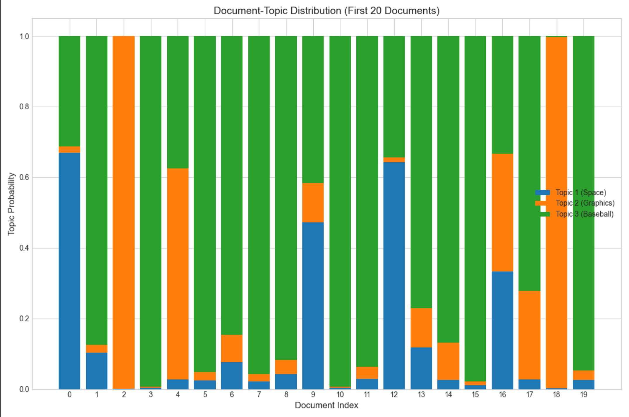
16.12 贝塔过程和印度自助餐

核心概念
贝塔过程(BP)是二值特征的非参数先验,"印度自助餐过程(IBP)" 是 BP 的直观比喻:
- 自助餐有无限道菜(对应特征);
- 每个顾客(数据点)选择若干道菜(特征),选菜的概率和菜被选的次数相关;
- 适合建模高维稀疏的二值特征(比如用户 - 物品交互)。
16.13 注释
1.本文所有代码基于 Python 3.8+,依赖库:numpy、scipy、matplotlib、seaborn、scikit-learn;
2.贝叶斯估计的核心是 "概率思维",而非复杂公式,新手先理解共轭先验和后验更新的逻辑;
3.非参数贝叶斯(DP、GP、IBP)是进阶内容,建议先掌握参数贝叶斯再深入。
16.14 习题
- 修改 16.2.2 的贝塔分布代码,尝试 α=0.5, β=0.5 的先验(杰弗里斯先验),观察后验变化;
- 基于 16.3.1 的代码,尝试未知方差、已知均值的高斯分布贝叶斯估计;
- 用贝叶斯逻辑回归解决鸢尾花数据集的二分类问题;
- 对比贝叶斯 GMM 和普通 GMM 在少数据场景下的聚类效果。
16.15 参考文献
- 《机器学习导论》(Ethem Alpaydin 著)第 16 章;
- 《Pattern Recognition and Machine Learning》(Bishop 著)第 2、3、6 章;
- scikit-learn 官方文档:https://scikit-learn.org/stable/
总结

1.贝叶斯估计的核心是 "先验 + 似然→后验",共轭先验能大幅简化计算,是新手入门的关键;
2.离散分布用贝塔 / 狄利克雷先验,高斯分布用正态 / 逆伽马 / 逆威沙特先验,函数参数用高斯过程 / 贝叶斯回归;
3.贝叶斯的优势是能量化不确定性(置信区间、参数分布),模型比较和非参数建模是进阶方向。
所有代码均可直接复制运行(Mac 系统),建议动手修改参数,直观感受贝叶斯估计的魅力!如果有问题,欢迎在评论区交流~