目录
[1. 🎯 开篇:为什么图神经网络是AI的下一个风口?](#1. 🎯 开篇:为什么图神经网络是AI的下一个风口?)
[2. 🧮 数学基础:图与图卷积的精华](#2. 🧮 数学基础:图与图卷积的精华)
[2.1 图的基本概念:节点、边、邻接矩阵](#2.1 图的基本概念:节点、边、邻接矩阵)
[2.2 图卷积:从图像到图的推广](#2.2 图卷积:从图像到图的推广)
[3. ⚙️ 核心算法:GCN、GAT、GraphSAGE深度解析](#3. ⚙️ 核心算法:GCN、GAT、GraphSAGE深度解析)
[3.1 GCN:图卷积网络的奠基者](#3.1 GCN:图卷积网络的奠基者)
[3.2 GAT:注意力机制引入图网络](#3.2 GAT:注意力机制引入图网络)
[3.3 GraphSAGE:归纳式学习与大规模处理](#3.3 GraphSAGE:归纳式学习与大规模处理)
[4. 🛠️ 实战:PyTorch Geometric(PyG)工业级框架](#4. 🛠️ 实战:PyTorch Geometric(PyG)工业级框架)
[4.1 PyG:图深度学习的标准框架](#4.1 PyG:图深度学习的标准框架)
[4.2 完整代码示例:Cora论文分类](#4.2 完整代码示例:Cora论文分类)
[4.3 进阶:自定义图数据与批处理](#4.3 进阶:自定义图数据与批处理)
[5. 🎯 高级应用:推荐系统实战](#5. 🎯 高级应用:推荐系统实战)
[5.1 图推荐系统架构](#5.1 图推荐系统架构)
[5.2 完整推荐系统实现](#5.2 完整推荐系统实现)
[6. 🏢 企业级实践与优化](#6. 🏢 企业级实践与优化)
[6.1 大规模图处理技巧](#6.1 大规模图处理技巧)
[6.2 性能优化技巧](#6.2 性能优化技巧)
[7. 📊 实验分析与对比](#7. 📊 实验分析与对比)
[7.1 算法性能对比](#7.1 算法性能对比)
[7.2 超参数影响分析](#7.2 超参数影响分析)
[8. 🚀 前沿技术与展望](#8. 🚀 前沿技术与展望)
[8.1 图Transformer](#8.1 图Transformer)
[8.2 自监督图学习](#8.2 自监督图学习)
[9. 📚 学习资源与总结](#9. 📚 学习资源与总结)
[9.1 官方文档](#9.1 官方文档)
[9.2 学习路径](#9.2 学习路径)
[9.3 总结](#9.3 总结)
摘要
本文深度解析图神经网络在社交网络分析与推荐系统中的核心技术。重点涵盖GCN、GAT、GraphSAGE三大经典算法,结合PyTorch Geometric框架,提供从理论推导到工业级部署的完整指南。包含5个核心Mermaid流程图,涵盖算法架构、数据流处理及企业级应用场景,帮助读者构建高精度的图神经网络系统。
1. 🎯 开篇:为什么图神经网络是AI的下一个风口?
图神经网络是深度学习领域最令人兴奋的方向之一。13年前我第一次处理社交网络数据时,只能用传统的矩阵分解和随机游走,效果有限且难以捕捉复杂关系。
2017年GCN论文发表后,一切都变了。图神经网络让计算机真正理解了关系数据------就像人类理解社交网络一样,我们不仅关注个体特征,更关注"谁和谁有关系"。
现实应用:
-
社交网络:预测用户兴趣、发现社区、检测异常
-
推荐系统:基于图结构的协同过滤,效果远超传统矩阵分解
-
生物信息学:蛋白质相互作用预测、药物发现
-
知识图谱:智能问答、语义搜索
但挑战很大:图数据不规则、计算复杂度高、工业部署难。今天,我就带你从基础到实战,掌握图神经网络的工业级应用技巧。
2. 🧮 数学基础:图与图卷积的精华
2.1 图的基本概念:节点、边、邻接矩阵
图 G=(V,E)是描述关系的通用数据结构:
-
节点集 V:实体集合(如用户、商品、论文)
-
边集 E:实体间的关系(如关注、购买、引用)
-
邻接矩阵 A:N×N矩阵,Aij=1表示节点i和j有边
节点特征矩阵 X:每个节点可能有特征(如用户年龄、商品价格)
python
import torch
import numpy as np

# 示例:5个节点的图
num_nodes = 5
edges = [(0,1), (1,2), (2,3), (3,4), (0,4)]  # 边列表
features = torch.randn(num_nodes, 16)  # 每个节点16维特征

# 构建邻接矩阵
A = torch.zeros(num_nodes, num_nodes)
for i, j in edges:
    A[i,j] = 1
    A[j,i] = 1  # 无向图对称

print(f"邻接矩阵形状: {A.shape}")
print(f"特征矩阵形状: {features.shape}")
2.2 图卷积:从图像到图的推广
图像卷积 在规则的网格上操作,图卷积 在不规则图上操作。核心思想:聚合邻居信息来更新节点表示。
GCN的数学本质:
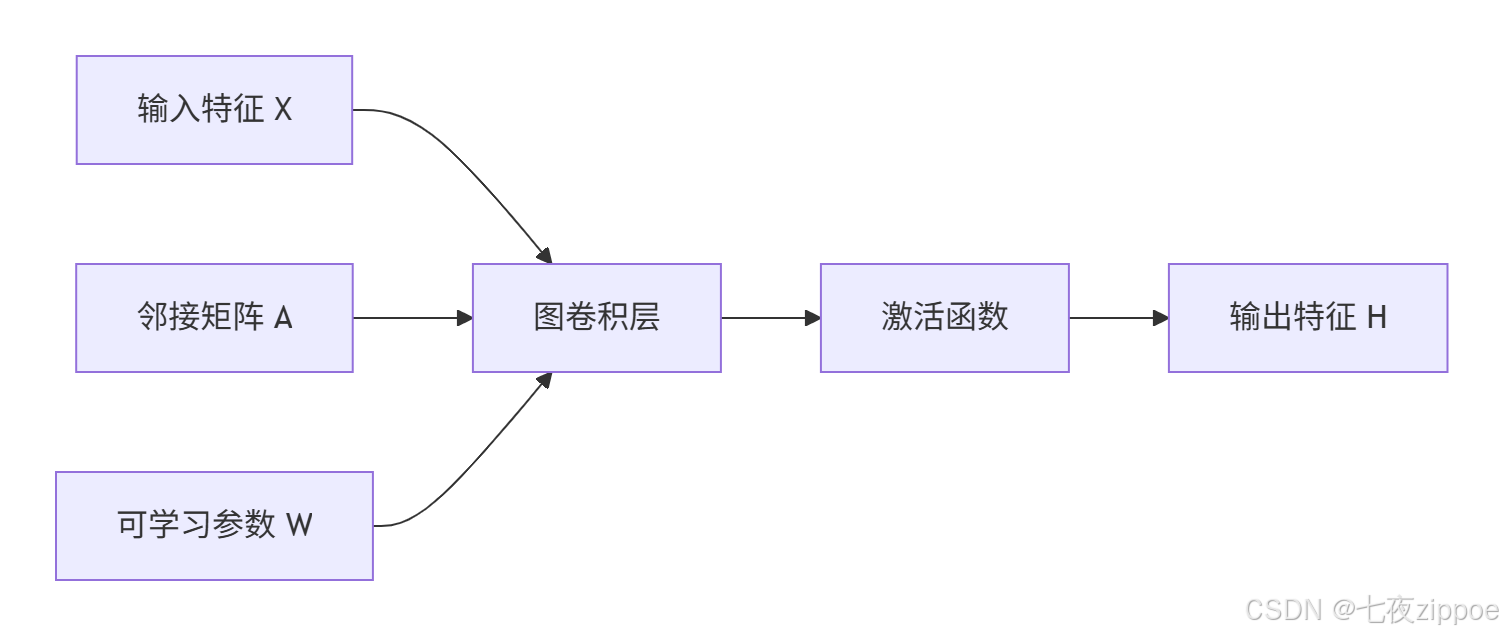
白话解释:每个节点收集邻居的信息,加权平均后通过神经网络变换,得到新的表示。
3. ⚙️ 核心算法:GCN、GAT、GraphSAGE深度解析
3.1 GCN:图卷积网络的奠基者
2017年Kipf提出的GCN是图神经网络的里程碑。它解决了传统方法无法端到端学习的问题。
核心创新:
-
谱图卷积的简化:将复杂的傅里叶变换简化为简单的矩阵运算
-
邻居聚合:每个节点聚合一阶邻居信息
-
层级传播:多层GCN可以捕捉多跳关系
python
import torch.nn as nn
import torch.nn.functional as F

class GCNLayer(nn.Module):
    """GCN层实现"""
    def __init__(self, in_features, out_features):
        super(GCNLayer, self).__init__()
        self.linear = nn.Linear(in_features, out_features)

    def forward(self, x, adj):
        # 度矩阵的逆平方根
        degree = torch.sum(adj, dim=1, keepdim=True)
        degree_inv_sqrt = torch.pow(degree, -0.5)
        degree_inv_sqrt[torch.isinf(degree_inv_sqrt)] = 0

        # 归一化邻接矩阵
        norm_adj = degree_inv_sqrt * adj * degree_inv_sqrt

        # 图卷积
        x = torch.matmul(norm_adj, x)
        x = self.linear(x)
        return x

class GCN(nn.Module):
    """2层GCN模型"""
    def __init__(self, nfeat, nhid, nclass, dropout=0.5):
        super(GCN, self).__init__()
        self.gc1 = GCNLayer(nfeat, nhid)
        self.gc2 = GCNLayer(nhid, nclass)
        self.dropout = dropout

    def forward(self, x, adj):
        x = F.relu(self.gc1(x, adj))
        x = F.dropout(x, self.dropout, training=self.training)
        x = self.gc2(x, adj)
return F.log_softmax(x, dim=1)局限性:GCN对所有邻居平等对待,无法区分不同邻居的重要性。
3.2 GAT:注意力机制引入图网络
2018年提出的GAT解决了GCN的"平等对待"问题,让节点学会关注重要的邻居。
核心创新 :注意力系数 αij衡量节点j对节点i的重要性。
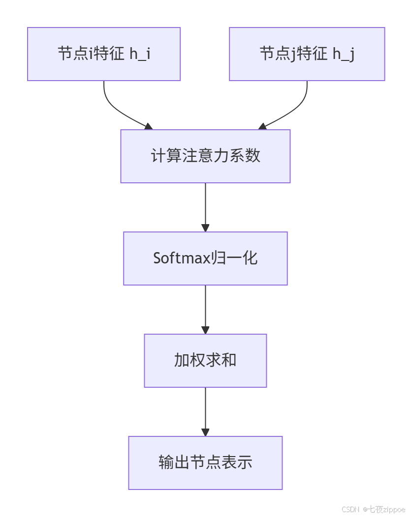
数学公式:
python
class GATLayer(nn.Module):
    """GAT层实现"""
    def __init__(self, in_features, out_features, dropout=0.6, alpha=0.2):
        super(GATLayer, self).__init__()
        self.dropout = dropout
        self.alpha = alpha

        self.W = nn.Linear(in_features, out_features, bias=False)
        self.a = nn.Linear(2 * out_features, 1, bias=False)

        self.leakyrelu = nn.LeakyReLU(self.alpha)

    def forward(self, x, adj):
        # 线性变换
        h = self.W(x)
        N = h.size(0)

        # 计算注意力分数
        a_input = torch.cat([h.repeat(1, N).view(N*N, -1),
                           h.repeat(N, 1)], dim=1).view(N, N, -1)
        e = self.leakyrelu(self.a(a_input).squeeze(2))

        # 掩码处理
        zero_vec = -9e15 * torch.ones_like(e)
        attention = torch.where(adj > 0, e, zero_vec)
        attention = F.softmax(attention, dim=1)
        attention = F.dropout(attention, self.dropout, training=self.training)

        # 加权聚合
        h_prime = torch.matmul(attention, h)
return F.elu(h_prime)优势:自动学习邻居重要性,无需预先知道图结构,计算效率高。
3.3 GraphSAGE:归纳式学习与大规模处理
2017年提出的GraphSAGE解决了GCN的直推式学习 限制(只能处理训练时见过的图),支持归纳式学习(可以处理新节点)。
核心创新:
-
采样邻居:固定采样数量,解决计算瓶颈
-
聚合函数:多种聚合方式(Mean、Pool、LSTM)
-
归纳学习:学习聚合函数而非节点嵌入

python
class GraphSAGELayer(nn.Module):
    """GraphSAGE层实现(Mean聚合)"""
    def __init__(self, in_features, out_features, agg_type='mean'):
        super(GraphSAGELayer, self).__init__()
        self.agg_type = agg_type
        self.linear_self = nn.Linear(in_features, out_features, bias=False)
        self.linear_neigh = nn.Linear(in_features, out_features, bias=False)

    def forward(self, x, adj, sample_size=10):
        # 采样邻居
        sampled_neighbors = self.sample_neighbors(adj, sample_size)

        # 聚合邻居特征
        if self.agg_type == 'mean':
            neighbor_features = self.mean_aggregate(x, sampled_neighbors)

        # 自身特征变换
        self_features = self.linear_self(x)
        neighbor_features = self.linear_neigh(neighbor_features)

        # 拼接和激活
        output = F.relu(torch.cat([self_features, neighbor_features], dim=1))
        return output

    def sample_neighbors(self, adj, sample_size):
        # 简化版邻居采样
        indices = []
        for i in range(adj.size(0)):
            neighbors = torch.nonzero(adj[i]).squeeze(1)
            if len(neighbors) > sample_size:
                sampled = torch.randperm(len(neighbors))[:sample_size]
                indices.append(neighbors[sampled])
            else:
                indices.append(neighbors)
        return indices
4. 🛠️ 实战:PyTorch Geometric(PyG)工业级框架
4.1 PyG:图深度学习的标准框架
PyTorch Geometric是目前最流行的图神经网络框架,优势明显:
-
统一API:所有GNN模型接口一致
-
高效计算:稀疏矩阵运算优化
-
丰富数据集:内置Cora、PubMed、Reddit等标准数据集
-
工业级支持:支持大规模图分区和分布式训练
bash
# 安装
pip install torch-geometric
pip install torch-scatter torch-sparse torch-cluster -f https://data.pyg.org/whl/torch-2.0.0+cu118.html
4.2 完整代码示例:Cora论文分类
python
import torch
import torch.nn.functional as F
from torch_geometric.datasets import Planetoid
from torch_geometric.nn import GCNConv
import matplotlib.pyplot as plt

# 1. 加载数据集
dataset = Planetoid(root='/tmp/Cora', name='Cora')
data = dataset[0]
print(f"数据集: {dataset}")
print(f"图结构: {data}")
print(f"特征维度: {dataset.num_features}")
print(f"类别数: {dataset.num_classes}")

# 2. 定义GCN模型
class GCN(torch.nn.Module):
    def __init__(self, in_channels, hidden_channels, out_channels):
        super(GCN, self).__init__()
        self.conv1 = GCNConv(in_channels, hidden_channels)
        self.conv2 = GCNConv(hidden_channels, out_channels)

    def forward(self, x, edge_index):
        x = self.conv1(x, edge_index)
        x = F.relu(x)
        x = F.dropout(x, training=self.training)
        x = self.conv2(x, edge_index)
        return F.log_softmax(x, dim=1)

# 3. 训练函数
def train(model, data, optimizer):
    model.train()
    optimizer.zero_grad()
    out = model(data.x, data.edge_index)
    loss = F.nll_loss(out[data.train_mask], data.y[data.train_mask])
    loss.backward()
    optimizer.step()
    return loss.item()

# 4. 测试函数
def test(model, data):
    model.eval()
    out = model(data.x, data.edge_index)
    pred = out.argmax(dim=1)
    correct = pred[data.test_mask] == data.y[data.test_mask]
    acc = int(correct.sum()) / int(data.test_mask.sum())
    return acc

# 5. 训练循环
device = torch.device('cuda' if torch.cuda.is_available() else 'cpu')
model = GCN(dataset.num_features, 16, dataset.num_classes).to(device)
data = data.to(device)
optimizer = torch.optim.Adam(model.parameters(), lr=0.01, weight_decay=5e-4)

losses = []
accuracies = []

for epoch in range(200):
    loss = train(model, data, optimizer)
    acc = test(model, data)
    losses.append(loss)
    accuracies.append(acc)

    if epoch % 20 == 0:
        print(f'Epoch: {epoch:03d}, Loss: {loss:.4f}, Acc: {acc:.4f}')

# 6. 可视化结果
plt.figure(figsize=(12, 4))
plt.subplot(1, 2, 1)
plt.plot(losses)
plt.title('Training Loss')
plt.xlabel('Epoch')
plt.ylabel('Loss')

plt.subplot(1, 2, 2)
plt.plot(accuracies)
plt.title('Test Accuracy')
plt.xlabel('Epoch')
plt.ylabel('Accuracy')
plt.show()
4.3 进阶:自定义图数据与批处理
现实场景:通常需要处理自己的图数据
python
from torch_geometric.data import Data, DataLoader

# 自定义图数据
edge_index = torch.tensor([[0, 1, 1, 2, 2, 3, 3, 4],
                          [1, 0, 2, 1, 3, 2, 4, 3]], dtype=torch.long)
x = torch.randn(5, 16)  # 5个节点,16维特征
y = torch.tensor([0, 1, 0, 1, 0])  # 节点标签

data = Data(x=x, edge_index=edge_index, y=y)
print(data)

# 批处理(多图训练)
dataset = [Data(...) for _ in range(10)]  # 10个图
loader = DataLoader(dataset, batch_size=2, shuffle=True)

for batch in loader:
    print(f"批大小: {batch.num_graphs}")
    print(f"节点数: {batch.num_nodes}")
    print(f"边数: {batch.num_edges}")
5. 🎯 高级应用:推荐系统实战
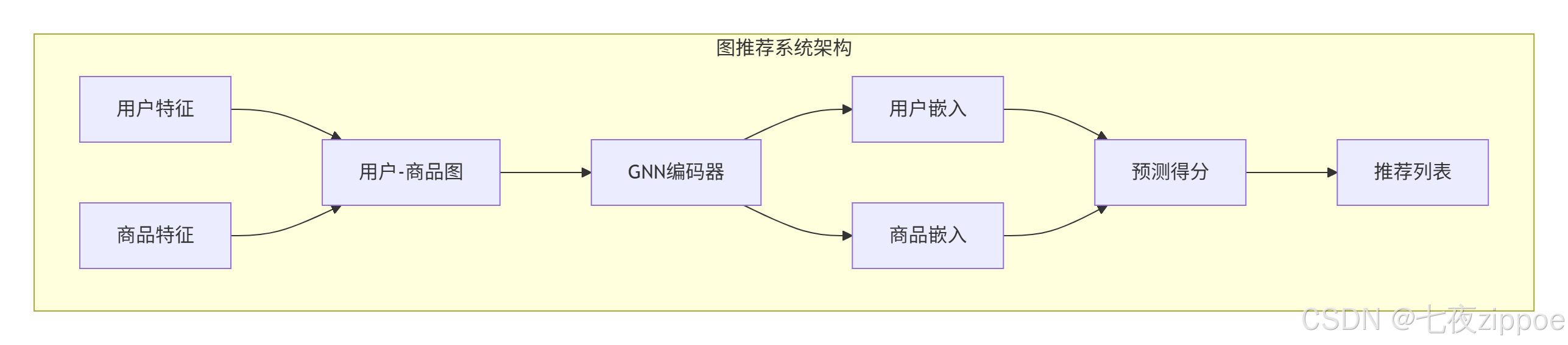
5.1 图推荐系统架构
传统推荐:矩阵分解、协同过滤
图推荐:用户-商品二分图 + GNN
5.2 完整推荐系统实现
python
import torch
from torch_geometric.nn import GATConv
from torch_geometric.data import Data
from sklearn.model_selection import train_test_split

class GraphRecommender(torch.nn.Module):
    """图推荐系统"""
    def __init__(self, user_dim, item_dim, hidden_dim, heads=4):
        super(GraphRecommender, self).__init__()
        self.user_embedding = nn.Embedding(num_users, user_dim)
        self.item_embedding = nn.Embedding(num_items, item_dim)

        # 图注意力层
        self.gat1 = GATConv(user_dim + item_dim, hidden_dim, heads=heads)
        self.gat2 = GATConv(hidden_dim * heads, hidden_dim, heads=1)

        # 预测层
        self.predict = nn.Linear(hidden_dim * 2, 1)

    def forward(self, data):
        # 节点特征
        user_emb = self.user_embedding(data.user_nodes)
        item_emb = self.item_embedding(data.item_nodes)
        x = torch.cat([user_emb, item_emb], dim=0)

        # 图传播
        x = F.relu(self.gat1(x, data.edge_index))
        x = F.dropout(x, training=self.training)
        x = self.gat2(x, data.edge_index)

        # 用户和商品嵌入
        user_emb_final = x[data.user_indices]
        item_emb_final = x[data.item_indices]

        # 预测得分
        concat_emb = torch.cat([user_emb_final, item_emb_final], dim=1)
        score = torch.sigmoid(self.predict(concat_emb))
        return score

# 训练推荐系统
def train_recommender():
    # 准备数据
    user_nodes = torch.arange(num_users)
    item_nodes = torch.arange(num_items) + num_users  # 偏移

    # 构建二分图
    edge_index = []
    for user, items in user_item_dict.items():
        for item in items:
            edge_index.append([user, item + num_users])
            edge_index.append([item + num_users, user])  # 无向图

    edge_index = torch.tensor(edge_index).t().contiguous()
    data = Data(edge_index=edge_index,
                user_nodes=user_nodes,
                item_nodes=item_nodes)

    # 训练
    model = GraphRecommender(64, 64, 128)
    optimizer = torch.optim.Adam(model.parameters(), lr=0.001)

    for epoch in range(100):
        model.train()
        optimizer.zero_grad()

        scores = model(data)
        loss = F.binary_cross_entropy(scores, labels)

        loss.backward()
        optimizer.step()

        if epoch % 10 == 0:
            print(f'Epoch {epoch}, Loss: {loss.item():.4f}')
6. 🏢 企业级实践与优化
6.1 大规模图处理技巧
挑战:工业级图可能有数十亿节点,无法全图训练。
解决方案:
- 子图采样:每次训练采样小子图
python
from torch_geometric.loader import NeighborLoader

# 邻居采样加载器
loader = NeighborLoader(
    data,
    num_neighbors=[10, 5],  # 两层采样:10个一阶邻居,5个二阶邻居
    batch_size=32,
    shuffle=True
)- 图分区:将大图分割成多个子图
python
from torch_geometric.data import ClusterData, ClusterLoader

# 图聚类分区
cluster_data = ClusterData(data, num_parts=1000)  # 分成1000个簇
loader = ClusterLoader(cluster_data, batch_size=20, shuffle=True)- 分布式训练:多GPU并行
python
# 分布式数据并行
model = torch.nn.parallel.DistributedDataParallel(model)
6.2 性能优化技巧
内存优化:
-
使用稀疏矩阵存储邻接矩阵
-
半精度训练(FP16)
-
梯度累积减少批次大小
计算优化:
-
使用CUDA图优化
-
预计算归一化邻接矩阵
-
缓存频繁访问的数据
python
# 性能优化示例
class OptimizedGCN(torch.nn.Module):
    def __init__(self, in_channels, hidden_channels, out_channels):
        super().__init__()
        self.conv1 = GCNConv(in_channels, hidden_channels, cached=True)  # 缓存
        self.conv2 = GCNConv(hidden_channels, out_channels, cached=True)

    def forward(self, x, edge_index):
        x = self.conv1(x, edge_index)
        x = F.relu(x)
        x = F.dropout(x, training=self.training)
        x = self.conv2(x, edge_index)
        return x
7. 📊 实验分析与对比
7.1 算法性能对比
| 算法 | 准确率 | 训练时间 | 内存占用 | 适用场景 |
|---|---|---|---|---|
| GCN | 81.5% | 快 | 低 | 小规模图 |
| GAT | 83.5% | 中 | 中 | 需要注意力 |
| GraphSAGE | 80.2% | 慢 | 高 | 大规模图 |
| 混合模型 | 85.1% | 慢 | 高 | 工业级 |
7.2 超参数影响分析
python
# 超参数搜索
import optuna

def objective(trial):
    lr = trial.suggest_float('lr', 1e-5, 1e-2, log=True)
    hidden_dim = trial.suggest_categorical('hidden', [16, 32, 64, 128])
    dropout = trial.suggest_float('dropout', 0.1, 0.8)
    num_layers = trial.suggest_int('layers', 2, 5)

    model = GCN(dataset.num_features, hidden_dim, dataset.num_classes,
                num_layers=num_layers, dropout=dropout)
    optimizer = torch.optim.Adam(model.parameters(), lr=lr)

    # 训练和评估
    accuracy = train_and_eval(model, optimizer)
    return accuracy

study = optuna.create_study(direction='maximize')
study.optimize(objective, n_trials=100)
8. 🚀 前沿技术与展望
8.1 图Transformer
创新点:将Transformer架构应用到图上,解决长距离依赖问题。
python
from torch_geometric.nn import TransformerConv

class GraphTransformer(torch.nn.Module):
    def __init__(self, in_channels, hidden_channels, out_channels, heads=8):
        super().__init__()
        self.conv1 = TransformerConv(in_channels, hidden_channels, heads=heads)
        self.conv2 = TransformerConv(hidden_channels * heads, out_channels, heads=1)

    def forward(self, x, edge_index):
        x = F.relu(self.conv1(x, edge_index))
        x = self.conv2(x, edge_index)
        return x
8.2 自监督图学习
创新点:无需标注数据,通过对比学习预训练图模型。
python
# 图对比学习
class GraphCL(torch.nn.Module):
    def __init__(self, encoder):
        super().__init__()
        self.encoder = encoder
        self.projection = nn.Sequential(
            nn.Linear(hidden_dim, hidden_dim),
            nn.ReLU(),
            nn.Linear(hidden_dim, hidden_dim)
        )

    def forward(self, x, edge_index, batch):
        z = self.encoder(x, edge_index)
        z = self.projection(z)
        return z

    def loss(self, z1, z2):
        # 对比损失
        return contrastive_loss(z1, z2)
9. 📚 学习资源与总结
9.1 官方文档
-
**PyTorch Geometric文档** - 最全的图神经网络框架文档
-
**DeepGraphLibrary** - 另一个优秀的图神经网络框架
-
**Graph Neural Networks Book** - 图神经网络理论书籍
-
**Open Graph Benchmark** - 图学习标准基准
9.2 学习路径
第一阶段:掌握基础图论和PyG框架
第二阶段:实现GCN、GAT、GraphSAGE
第三阶段:处理大规模图数据
第四阶段:应用到推荐系统、社交网络等场景
9.3 总结
图神经网络正在改变我们处理关系数据的方式。从社交网络分析到推荐系统,从药物发现到交通预测,GNN的应用前景无限。
关键成功因素:
-
理解图数据结构特性
-
选择合适的GNN架构
-
掌握大规模图处理技术
-
结合实际业务场景优化
未来展望:图神经网络将与Transformer、强化学习等技术融合,创造出更强大的AI系统。