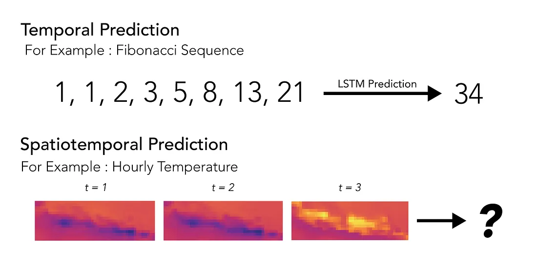
In time series data, there are several tasks that are commonly performed, such as classification, event detection, anomaly detection, and the most dominant task is forecasting. Forecasting is simply predicting future information by utilizing information from the present and past. This is possible by assuming that time series data are correlated with each other or autocorrelated. In deep learning or neural networks, this assumption is utilized in the creation of architectures such as Long-Short Term Memory (LSTM) and Gated Recurrent Unit (GRU). Both of these architectures are part of the Recurrent Neural Network (RNN).
In the application, RNN can predict future information (Forecasting) in the form of a sequence by utilizing a sequence of current and past information. However, problems arise if the information we want to get is in the form of a spatial sequence. So the question comes up, can neural networks be applied to the prediction of spatiotemporal data?
Results of CNN and RNN Combination
Unlike RNN that can capture time patterns, Convolutional Neural Network is very good at capturing spatial patterns. This is because CNN allows the extraction of spatial features into complex and abstract features by utilizing the Convolution layer.
By utilizing algorithms from CNN and RNN, an architecture called ConvLSTM was born. ConvLSTM is simply an algorithm that integrates convolution elements into the LSTM architecture so that it is possible to extract spatial features first and then extract the time series pattern. This allows for spatiotemporal data to be predicted over time. However, ConvLSTM is better for nowcasting or forecasting in a short time (not too long).
Example : Java Region Hourly Temperature Nowcasting
To demonstrate ConvLSTM there are several data that can be used such as video data and climate data. In this article, climate data in the form of Hourly Temperature in the Java Island region of Indonesia is used for nowcasting. The objective of this example is to create a model that allows predicting 12 hours of temperature data by utilizing data from the previous 12 hours.
Steps of Analysis
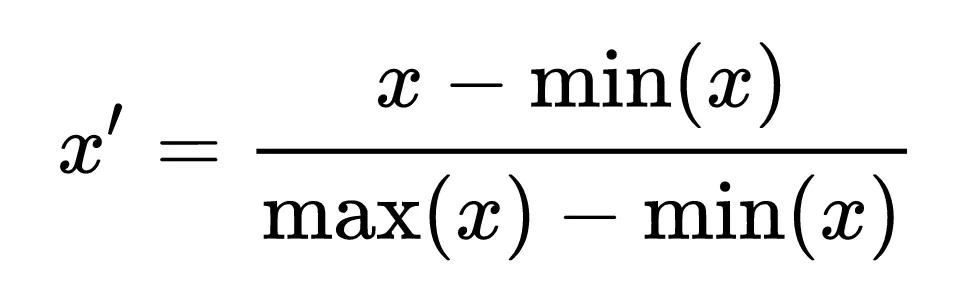
Normalization
The first thing done to the data is normalization. This is done to constrain the value to be between 0 and 1. Normalization is done on temperature data so that it can be treated as video data using a min-max scaler.
Press enter or click to view image in full size
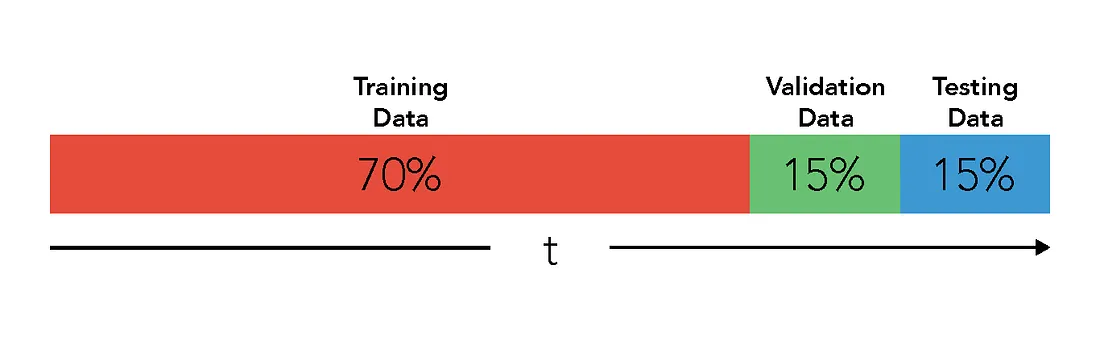
Data Splitting
As in machine learning models, the data is divided into train, validation, and test. 70% of the initial data is used as train data, 15% of the next data for validation, and the remaining 15% for test.
Reshaping
To be able to use ConvLSTM architecture specifically ConvLSTM2D, input and output data needs to be converted into 5D tensor with the following details (num_samples, num_timesteps, num_longitudes, num_latitudes, num_features) . Where num_samples is the total number of samples, num_timesteps is the number of sequences in each sample, num_longitudes is the number of longitudes or number of rows, num_latitudes is the number of longitudes or number of columns, and num_features is the number of features or channels.
In this problem, the output data is shifted by one from the input data. This means that if the input starts from time t then the output starts from time t+1. This is done because the model produced is better than the output data only in the form of spatial data with a time dimension of one.
Train The ConvLSTM
The architecture used is 3 stacked ConvLSTM2D layers plus Conv3D output layer with an alternating Batch Normalization layer in each layer. The architecture in Python syntax can be seen below.
python
from tensorflow import keras
from tensorflow.keras import layers
inp = layers.Input(shape=(None, num_longitudes, num_latitudes, num_features))
x = layers.BatchNormalization()(inp)
x = layers.ConvLSTM2D(
filters=16,
kernel_size=(5, 5),
padding="same",
return_sequences=True,
activation="relu",
)(x)
x = layers.BatchNormalization()(x)
x = layers.ConvLSTM2D(
filters=32,
kernel_size=(3, 3),
padding="same",
return_sequences=True,
activation="relu",
)(x)
x = layers.BatchNormalization()(x)
x = layers.BatchNormalization()(x)
x = layers.ConvLSTM2D(
filters=32,
kernel_size=(1, 1),
padding="same",
return_sequences=True,
activation="relu",
)(x)
x = layers.BatchNormalization()(x)
x = layers.Conv3D(
filters=1, kernel_size=(3, 3, 3), activation="sigmoid", padding="same"
)(x)
model = keras.models.Model(inp, x)
model.compile(
loss=keras.losses.binary_crossentropy, optimizer=keras.optimizers.Adam(),
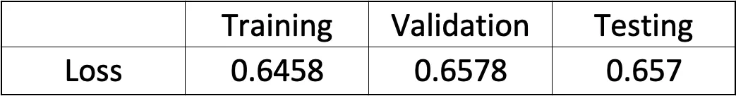
)The hyperparameters in this model are the results of hyperparameter tuning using the Hyperband method. After that, training is carried out and the loss for each part of the data is obtained as follows.
Prediction
After the best model has been obtained, then we try to do a 12-hour prediction with the data that has been displayed previously. After that, it is compared with the actual value or ground truth of what we predict.
It can be seen that ConvLSTM can be said to be good enough in making predictions in a short period (Nowcasting). The predicted value can be seen to follow the temperature pattern and also the temperature value even though the prediction results look blurry.
Restriction
Apart from the ability of ConvLSTM to predict spatiotemporal in the short term. The architecture used has a restriction that the predicted value cannot be more than the maximum value and below the minimum value in the training data. This is because we use min-max scaler for data normalization so that if the data we predict has anomalies, the architecture currently used cannot capture it.
Conclusion
ConvLSTM is a method that can be used to predict spatiotemporal values for short time periods. There are many applications with this method, one of which is in the field of climate as in the example in this article with quite usable results.