RNN 循环神经网络 计算过程(通俗+公式版)
RNN 的核心是对序列数据按时间步依次计算,每个时刻都复用同一套权重,并把上一时刻的状态传给下一时刻。
1. 符号定义
-xt\Large x_txt :第t\Large tt 时刻输入
-ht−1\Large h_{t-1}ht−1 :上一时刻隐藏状态
-ht\Large h_tht :当前时刻隐藏状态
-Wxh\Large W_{xh}Wxh :输入到隐藏层权重
-Whh\Large W_{hh}Whh :隐藏层自循环权重
-bh\Large b_hbh :隐藏层偏置
-Why\Large W_{hy}Why :隐藏到输出权重
-by\Large b_yby :输出偏置
-tanh\Large \tanhtanh :激活函数
2. 单步计算流程
对每个时间步t\Large tt :
① 计算隐藏状态
ht=tanh(Wxhxt+Whhht−1+bh) \Large h_t = \tanh\big(W_{xh} x_t + W_{hh} h_{t-1} + b_h\big) ht=tanh(Wxhxt+Whhht−1+bh)
- 初始状态:h0=0\Large h_0 = \mathbf{0}h0=0 (全零向量)
② 计算输出
yt=Whyht+by \Large y_t = W_{hy} h_t + b_y yt=Whyht+by
(分类任务后接 softmax,回归任务直接输出)
3. 完整前向传播(序列展开)
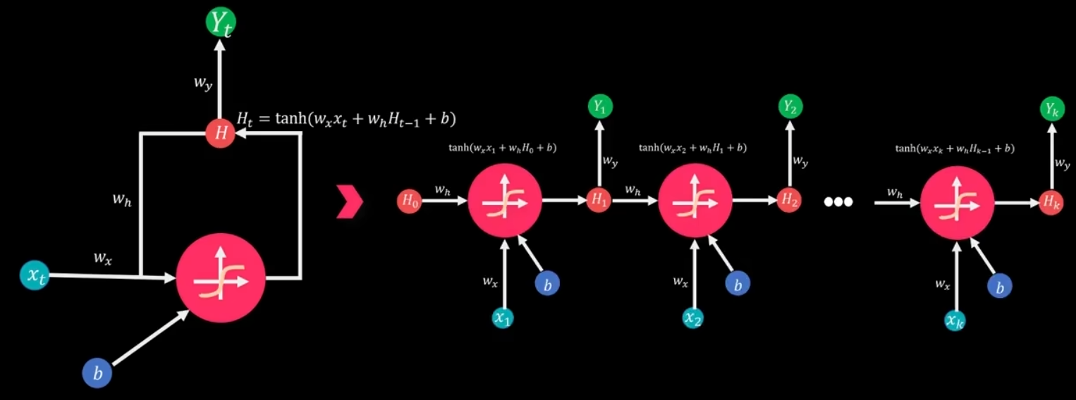
给定序列x1,x2,...,xT\Large x_1,x_2,\dots,x_Tx1,x2,...,xT :
1.t=1\Large t=1t=1
h1=tanh(Wxhx1+Whhh0+bh),y1=Whyh1+by \Large h_1 = \tanh(W_{xh}x_1 + W_{hh}h_0 + b_h),\quad y_1 = W_{hy}h_1 + b_y h1=tanh(Wxhx1+Whhh0+bh),y1=Whyh1+by
2.t=2\Large t=2t=2
h2=tanh(Wxhx2+Whhh1+bh),y2=Whyh2+by \Large h_2 = \tanh(W_{xh}x_2 + W_{hh}h_1 + b_h),\quad y_2 = W_{hy}h_2 + b_y h2=tanh(Wxhx2+Whhh1+bh),y2=Whyh2+by
- 一直重复到t=T\Large t=Tt=T
hT=tanh(WxhxT+WhhhT−1+bh),yT=WhyhT+by\Large h_T = \tanh(W_{xh}x_T + W_{hh}h_{T-1} + b_h),\quad y_T = W_{hy}h_T + b_yhT=tanh(WxhxT+WhhhT−1+bh),yT=WhyhT+by
关键 :所有权重Wxh,Whh,Why\Large W_{xh},W_{hh},W_{hy}Wxh,Whh,Why 在所有时间步共享。
4. 反向传播 BPTT 要点
- 损失:L=∑t=1TLt(yt,y^t)\Large L = \sum_{t=1}^T L_t(y_t, \hat{y}_t)L=∑t=1TLt(yt,y^t)
- 梯度沿时间反向传播,对Wxh,Whh,Why\Large W_{xh},W_{hh},W_{hy}Wxh,Whh,Why 求导并累加
- 容易出现梯度消失/爆炸,所以后来才有 LSTM、GRU
5. 极简总结
RNN 就是:
输入 + 上一时刻状态 → 激活 → 当前状态 → 输出
一步一步沿着序列走,权重全程不变。
好,我们直接来一个标准矩阵版 RNN 手算例子,维度小、步骤全,能看清每一步矩阵运算。
1. 设定参数
- 输入维度:dx=2d_x = 2dx=2
- 隐藏层维度:dh=2d_h = 2dh=2
- 输出维度:dy=1d_y = 1dy=1
- 序列长度 T=2T=2T=2,输入:
x1=10,x2=01 \Large x_1=\begin{bmatrix}1\\0\end{bmatrix},\quad x_2=\begin{bmatrix}0\\1\end{bmatrix} x1= 10 ,x2= 01 - 初始隐藏状态:
h0=00 h_0 = \begin{bmatrix}0\\0\end{bmatrix} h0=00
权重矩阵(手动给定)
Wxh=0.10.20.30.4,Whh=0.50.60.70.8,bh=0.10.2 \Large W_{xh} = \begin{bmatrix} 0.1 & 0.2\\ 0.3 & 0.4 \end{bmatrix},\quad W_{hh} = \begin{bmatrix} 0.5 & 0.6\\ 0.7 & 0.8 \end{bmatrix},\quad b_h = \begin{bmatrix}0.1\\0.2\end{bmatrix} Wxh= 0.10.30.20.4 ,Whh= 0.50.70.60.8 ,bh= 0.10.2
Why=0.91.0,by=0.1 \Large W_{hy} = \begin{bmatrix}0.9 & 1.0\end{bmatrix},\quad b_y = 0.1 Why=0.91.0,by=0.1
激活函数:tanh\tanhtanh
2. 计算公式
ht=tanh(Wxhxt+Whhht−1+bh) \Large h_t = \tanh\left(W_{xh}x_t + W_{hh}h_{t-1} + b_h\right) ht=tanh(Wxhxt+Whhht−1+bh)
yt=Whyht+by \Large y_t = W_{hy}h_t + b_y yt=Whyht+by
3. 计算 t=1
- 线性部分
Wxhx1=0.10.20.30.410=0.10.3 \Large W_{xh}x_1 = \begin{bmatrix}0.1&0.2\\0.3&0.4\end{bmatrix}\begin{bmatrix}1\\0\end{bmatrix} = \begin{bmatrix}0.1\\0.3\end{bmatrix} Wxhx1= 0.10.30.20.4 10 = 0.10.3
Whhh0=0 \Large W_{hh}h_0 = 0 Whhh0=0
z1=Wxhx1+Whhh0+bh=0.10.3+0.10.2=0.20.5 \Large z_1 = W_{xh}x_1 + W_{hh}h_0 + b_h = \begin{bmatrix}0.1\\0.3\end{bmatrix} + \begin{bmatrix}0.1\\0.2\end{bmatrix} = \begin{bmatrix}0.2\\0.5\end{bmatrix} z1=Wxhx1+Whhh0+bh= 0.10.3 + 0.10.2 = 0.20.5
- 激活
h1=tanh0.20.5≈0.1970.462 \Large h_1 = \tanh\begin{bmatrix}0.2\\0.5\end{bmatrix} \approx \begin{bmatrix}0.197\\0.462\end{bmatrix} h1=tanh 0.20.5 ≈ 0.1970.462 - 输出
y1=0.91.00.1970.462+0.1≈0.177+0.462+0.1=0.739 \Large y_1 = \begin{bmatrix}0.9&1.0\end{bmatrix}\begin{bmatrix}0.197\\0.462\end{bmatrix} + 0.1 \approx 0.177 + 0.462 + 0.1 = 0.739 y1=0.91.0 0.1970.462 +0.1≈0.177+0.462+0.1=0.739
4. 计算 t=2
- 线性部分
Wxhx2=0.10.20.30.401=0.20.4 \Large W_{xh}x_2 = \begin{bmatrix}0.1&0.2\\0.3&0.4\end{bmatrix}\begin{bmatrix}0\\1\end{bmatrix} = \begin{bmatrix}0.2\\0.4\end{bmatrix} Wxhx2= 0.10.30.20.4 01 = 0.20.4
Whhh1=0.50.60.70.80.1970.462≈0.3760.507 \Large W_{hh}h_1 =\begin{bmatrix}0.5&0.6\\0.7&0.8\end{bmatrix}\begin{bmatrix}0.197\\0.462\end{bmatrix} \approx\begin{bmatrix}0.376\\0.507\end{bmatrix} Whhh1= 0.50.70.60.8 0.1970.462 ≈ 0.3760.507
z2=0.20.4+0.3760.507+0.10.2=0.6761.107 \Large z_2 = \begin{bmatrix}0.2\\0.4\end{bmatrix} +\begin{bmatrix}0.376\\0.507\end{bmatrix} +\begin{bmatrix}0.1\\0.2\end{bmatrix} = \begin{bmatrix}0.676\\1.107\end{bmatrix} z2= 0.20.4 + 0.3760.507 + 0.10.2 = 0.6761.107
- 激活
h2=tanh0.6761.107≈0.5880.803 \Large h_2 = \tanh\begin{bmatrix}0.676\\1.107\end{bmatrix} \approx\begin{bmatrix}0.588\\0.803\end{bmatrix} h2=tanh 0.6761.107 ≈ 0.5880.803 - 输出
y2=0.91.00.5880.803+0.1≈0.529+0.803+0.1=1.432 \Large y_2 = \begin{bmatrix}0.9&1.0\end{bmatrix}\begin{bmatrix}0.588\\0.803\end{bmatrix}+0.1 \approx 0.529+0.803+0.1 =1.432 y2=0.91.0 0.5880.803 +0.1≈0.529+0.803+0.1=1.432
5. 最终结果
h1≈0.1970.462, y1≈0.739 \Large h_1\approx\begin{bmatrix}0.197\\0.462\end{bmatrix},\ y_1\approx0.739 h1≈ 0.1970.462 , y1≈0.739
h2≈0.5880.803, y2≈1.432 \Large h_2\approx\begin{bmatrix}0.588\\0.803\end{bmatrix},\ y_2\approx1.432 h2≈ 0.5880.803 , y2≈1.432
6. 矩阵版 RNN 核心要点
- 每一步都是矩阵乘法 + 向量加法
- Wxh,Whh,WhyW_{xh},W_{hh},W_{hy}Wxh,Whh,Why 在所有时间步完全共享
- 隐藏状态 hth_tht 是向量,负责携带历史信息
- 计算是串行 的:必须先算 h1h_1h1 才能算 h2h_2h2