Day 11 编程实战：XGBoost金融预测与调参

Day 11 编程实战：XGBoost金融预测与调参

实战目标

1. 理解XGBoost的核心原理和参数
2. 使用XGBoost进行涨跌预测
3. 系统地进行参数调优
4. 对比XGBoost与随机森林、GBDT
5. 学习LightGBM的基本使用

1. 导入必要的库

import numpy as np
import pandas as pd
import matplotlib.pyplot as plt
import seaborn as sns
import time
from pathlib import Path
import warnings
warnings.filterwarnings('ignore')

# XGBoost和LightGBM
import xgboost as xgb
import lightgbm as lgb

# sklearn组件
from sklearn.model_selection import train_test_split, TimeSeriesSplit, GridSearchCV, RandomizedSearchCV
from sklearn.metrics import (
    accuracy_score, precision_score, recall_score, f1_score,
    roc_auc_score, roc_curve, classification_report, confusion_matrix
)
from sklearn.ensemble import RandomForestClassifier, GradientBoostingClassifier
from sklearn.preprocessing import StandardScaler

#启用LaTeX渲染（如果系统安装了LaTeX）
plt.rcParams['text.usetex'] = False  # 设为False避免LaTeX依赖
# 设置中文显示
plt.rcParams['font.sans-serif'] = ['SimHei', 'Microsoft YaHei', 'DejaVu Sans']
plt.rcParams['axes.unicode_minus'] = False

print("库导入成功！")
print(f"XGBoost版本: {xgb.__version__}")
print(f"LightGBM版本: {lgb.__version__}")

库导入成功！
XGBoost版本: 3.0.5
LightGBM版本: 4.6.0

2. 生成金融数据

def generate_financial_data(ts_code):
    """生成金融数据"""
    
    data_path = Path(r"E:\AppData\quant_trade\klines\kline2014-2024")
    kline_file = data_path / f"{ts_code}.csv"
    
    df = pd.read_csv(kline_file, usecols=["trade_date", "close", "vol"],
                     parse_dates=["trade_date"])\
            .rename(columns={"vol": "volume"})\
            .sort_values(by=["trade_date"])\
            .reset_index(drop=True)
    
    df['return'] = df['close'].pct_change()
    
    # 技术指标
    # RSI
    delta = df['return'].fillna(0)
    gain = delta.where(delta > 0, 0).rolling(14).mean()
    loss = -delta.where(delta < 0, 0).rolling(14).mean()
    rs = gain / (loss + 1e-10)
    df['rsi'] = 100 - (100 / (1 + rs))
    
    # MACD
    ema12 = df['close'].ewm(span=12, adjust=False).mean()
    ema26 = df['close'].ewm(span=26, adjust=False).mean()
    df['macd'] = ema12 - ema26
    df['macd_signal'] = df['macd'].ewm(span=9, adjust=False).mean()
    
    # 均线比率
    df['ma5'] = df['close'].rolling(5).mean()
    df['ma20'] = df['close'].rolling(20).mean()
    df['ma_ratio'] = df['ma5'] / df['ma20'] - 1
    
    # 波动率
    df['volatility'] = df['return'].rolling(20).std()
    
    # 成交量比率
    df['volume_ratio'] = df['volume'] / df['volume'].rolling(10).mean()
    
    # 动量指标
    for lag in [1, 2, 3, 5, 10]:
        df[f'momentum_{lag}'] = df['return'].shift(lag).fillna(0)
    
    # 目标变量：5日收盘是否上涨
    df['target'] = (df['close'].shift(-5) > df['close']).astype(int)
    
    # 删除缺失值
    df = df.dropna()
    
    return df

# 生成数据
ts_code = "300033.SZ"
df = generate_financial_data(ts_code)
print(f"数据形状: {df.shape}")

# 特征选择
feature_cols = ['rsi', 'macd', 'macd_signal', 'ma_ratio', 'volatility', 
                'volume_ratio', 'momentum_1', 'momentum_2', 'momentum_3', 
                'momentum_5', 'momentum_10']
X = df[feature_cols]
y = df['target']

print(f"特征数量: {len(feature_cols)}")
print(f"样本数量: {len(X)}")
print(f"目标分布: {y.value_counts(normalize=True)}")

# 按时间划分
split_idx = int(len(X) * 0.7)
X_train = X[:split_idx]
X_test = X[split_idx:]
y_train = y[:split_idx]
y_test = y[split_idx:]

print(f"\n训练集: {len(X_train)} 样本")
print(f"测试集: {len(X_test)} 样本")

# 标准化（随机森林不需要，但为了对比，依然做标准化）
scaler = StandardScaler()
X_train_scaled = scaler.fit_transform(X_train)
X_test_scaled = scaler.transform(X_test)

数据形状: (2451, 18)
特征数量: 11
样本数量: 2451
目标分布: target
1    0.504284
0    0.495716
Name: proportion, dtype: float64

训练集: 1715 样本
测试集: 736 样本

3. XGBoost基础模型

3.1 使用默认参数训练

print("="*60)
print("XGBoost默认参数模型")
print("="*60)

# 默认参数的XGBoost
xgb_default = xgb.XGBClassifier(
    n_estimators=100,
    learning_rate=0.3,
    max_depth=6,
    random_state=42,
    n_jobs=-1,
    eval_metric='logloss'
)

start_time = time.time()
xgb_default.fit(X_train, y_train)
train_time = time.time() - start_time

# 预测
y_pred_default = xgb_default.predict(X_test)
y_proba_default = xgb_default.predict_proba(X_test)[:, 1]

print(f"训练时间: {train_time:.2f}秒")
print(f"准确率: {accuracy_score(y_test, y_pred_default):.4f}")
print(f"精确率: {precision_score(y_test, y_pred_default):.4f}")
print(f"召回率: {recall_score(y_test, y_pred_default):.4f}")
print(f"F1: {f1_score(y_test, y_pred_default):.4f}")
print(f"AUC: {roc_auc_score(y_test, y_proba_default):.4f}")

============================================================
XGBoost默认参数模型
============================================================
训练时间: 0.11秒
准确率: 0.5815
精确率: 0.5553
召回率: 0.6029
F1: 0.5781
AUC: 0.5910

3.2 特征重要性分析

# 获取特征重要性
importances_xgb = xgb_default.feature_importances_
importance_df = pd.DataFrame({
    'feature': feature_cols,
    'importance': importances_xgb
}).sort_values('importance', ascending=False)

plt.figure(figsize=(10, 6))
plt.barh(importance_df['feature'], importance_df['importance'])
plt.xlabel('重要性')
plt.title('XGBoost特征重要性')
for i, (_, row) in enumerate(importance_df.iterrows()):
    plt.text(row['importance'] + 0.002, i, f"{row['importance']:.4f}", va='center')
plt.gca().invert_yaxis()
plt.grid(True, alpha=0.3)
plt.tight_layout()
plt.show()

print("特征重要性排序:")
print(importance_df.to_string(index=False))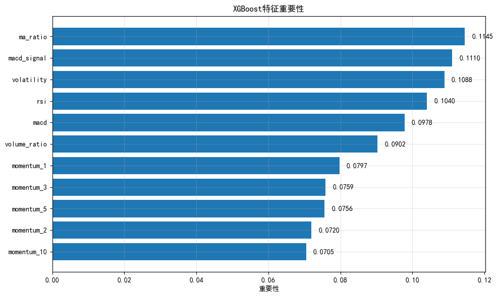

特征重要性排序:
     feature  importance
    ma_ratio    0.114539
 macd_signal    0.111010
  volatility    0.108831
         rsi    0.103969
        macd    0.097773
volume_ratio    0.090239
  momentum_1    0.079729
  momentum_3    0.075898
  momentum_5    0.075574
  momentum_2    0.071970
 momentum_10    0.070468

4. 单参数影响分析

4.1 max_depth的影响

def analyze_max_depth(X_train, y_train, X_test, y_test, depth_range=range(3, 13, 2)):
    """分析max_depth对模型性能的影响"""
    train_scores = []
    test_scores = []
    
    for depth in depth_range:
        model = xgb.XGBClassifier(
            n_estimators=100,
            learning_rate=0.3,
            max_depth=depth,
            random_state=42,
            n_jobs=-1
        )
        model.fit(X_train, y_train)
        
        train_scores.append(accuracy_score(y_train, model.predict(X_train)))
        test_scores.append(accuracy_score(y_test, model.predict(X_test)))
    
    plt.figure(figsize=(10, 6))
    plt.plot(depth_range, train_scores, 'b-o', label='训练集', linewidth=2, markersize=8)
    plt.plot(depth_range, test_scores, 'r-s', label='测试集', linewidth=2, markersize=8)
    plt.xlabel('max_depth')
    plt.ylabel('准确率')
    plt.title('max_depth对XGBoost性能的影响')
    plt.legend()
    plt.grid(True, alpha=0.3)
    
    best_depth = depth_range[np.argmax(test_scores)]
    plt.axvline(x=best_depth, color='g', linestyle='--', label=f'最佳={best_depth}')
    plt.legend()
    plt.show()
    
    print(f"最佳max_depth: {best_depth}")
    print(f"最佳测试准确率: {max(test_scores):.4f}")
    
    return best_depth

best_depth = analyze_max_depth(X_train, y_train, X_test, y_test)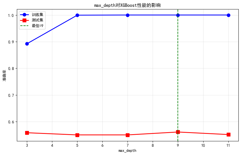

最佳max_depth: 9
最佳测试准确率: 0.5611

4.2 learning_rate的影响

def analyze_learning_rate(X_train, y_train, X_test, y_test, lr_range=[0.01, 0.05, 0.07, 0.09, 0.13, 0.15, 0.2]):
    """分析学习率对模型性能的影响"""
    train_scores = []
    test_scores = []
    
    for lr in lr_range:
        model = xgb.XGBClassifier(
            n_estimators=100,
            learning_rate=lr,
            max_depth=best_depth,
            random_state=42,
            n_jobs=-1
        )
        model.fit(X_train, y_train)
        
        train_scores.append(accuracy_score(y_train, model.predict(X_train)))
        test_scores.append(accuracy_score(y_test, model.predict(X_test)))
    
    plt.figure(figsize=(10, 6))
    plt.plot(lr_range, train_scores, 'b-o', label='训练集', linewidth=2, markersize=8)
    plt.plot(lr_range, test_scores, 'r-s', label='测试集', linewidth=2, markersize=8)
    plt.xscale('log')
    plt.xlabel('学习率 (learning_rate)')
    plt.ylabel('准确率')
    plt.title('学习率对XGBoost性能的影响')
    plt.legend()
    plt.grid(True, alpha=0.3)
    
    best_lr = lr_range[np.argmax(test_scores)]
    plt.axvline(x=best_lr, color='g', linestyle='--', label=f'最佳={best_lr}')
    plt.legend()
    plt.show()
    
    print(f"最佳learning_rate: {best_lr}")
    print(f"最佳测试准确率: {max(test_scores):.4f}")
    
    return best_lr

best_lr = analyze_learning_rate(X_train, y_train, X_test, y_test)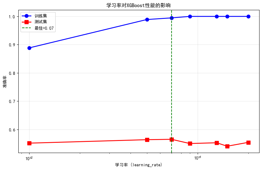

最佳learning_rate: 0.07
最佳测试准确率: 0.5652

4.3 n_estimators的影响与早停

def analyze_n_estimators_with_early_stop(X_train, y_train, X_val, y_val, max_trees=500):
    """分析树数量并演示早停"""
    
    # 使用早停训练
    model = xgb.XGBClassifier(
        n_estimators=max_trees,
        learning_rate=best_lr/10,
        max_depth=best_depth,
        early_stopping_rounds=20,
        eval_metric='logloss',
        random_state=42,
        n_jobs=-1
    )
    
    # 训练并记录评估历史
    model.fit(
        X_train, y_train,
        eval_set=[(X_val, y_val)],
        verbose=False
    )
    
    # 获取最佳迭代次数
    best_n = model.best_iteration
    best_score = model.best_score
    
    print(f"早停结果:")
    print(f"  最佳树数量: {best_n}")
    print(f"  最佳验证集AUC: {best_score:.4f}")
    
    # 可视化训练过程
    results = model.evals_result()
    
    plt.figure(figsize=(10, 6))
    plt.plot(results['validation_0']['logloss'], 'b-', label='验证集损失', linewidth=2)
    plt.xlabel('迭代次数')
    plt.ylabel('Log Loss')
    plt.title('XGBoost早停训练过程')
    plt.axvline(x=best_n, color='r', linestyle='--', label=f'早停点 (n={best_n})')
    plt.legend()
    plt.grid(True, alpha=0.3)
    plt.show()
    
    return best_n

# 划分验证集
split_val = int(len(X_train) * 0.8)
X_train_sub = X_train[:split_val]
y_train_sub = y_train[:split_val]
X_val = X_train[split_val:]
y_val = y_train[split_val:]

best_n = analyze_n_estimators_with_early_stop(X_train_sub, y_train_sub, X_val, y_val)

早停结果:
  最佳树数量: 64
  最佳验证集AUC: 0.6812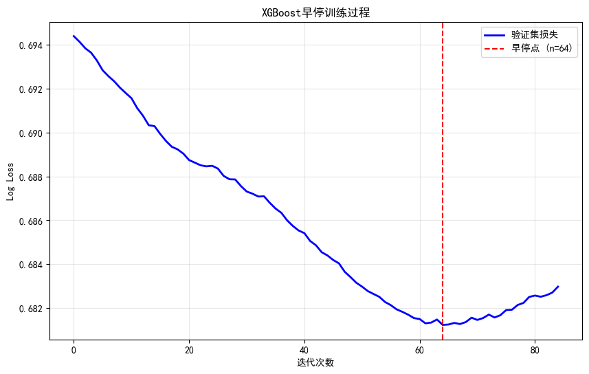

5. 网格搜索调参

5.1 第一阶段：调树结构参数

def grid_search_phase1(X_train, y_train):
    """第一阶段：调max_depth和min_child_weight"""
    
    # 参数网格
    param_grid = {
        'max_depth': [3, 5, 7, 9],
        'min_child_weight': [1, 3, 5, 7]
    }
    
    # 基础模型（固定学习率）
    base_model = xgb.XGBClassifier(
        n_estimators=100,
        learning_rate=0.3,
        random_state=42,
        n_jobs=-1,
        eval_metric='logloss'
    )
    
    # 时间序列交叉验证
    tscv = TimeSeriesSplit(n_splits=3)
    
    grid_search = GridSearchCV(
        base_model, param_grid,
        cv=tscv,
        scoring='roc_auc',
        n_jobs=-1,
        verbose=1
    )
    
    print("第一阶段网格搜索（树结构参数）...")
    start_time = time.time()
    grid_search.fit(X_train, y_train)
    elapsed = time.time() - start_time
    
    print(f"\n搜索完成，耗时: {elapsed:.2f}秒")
    print(f"最佳参数: {grid_search.best_params_}")
    print(f"最佳CV AUC: {grid_search.best_score_:.4f}")
    
    return grid_search.best_params_

# 执行第一阶段搜索
best_params_phase1 = grid_search_phase1(X_train, y_train)

第一阶段网格搜索（树结构参数）...
Fitting 3 folds for each of 16 candidates, totalling 48 fits

搜索完成，耗时: 4.16秒
最佳参数: {'max_depth': 9, 'min_child_weight': 7}
最佳CV AUC: 0.5055

5.2 第二阶段：调学习率和树数量

def grid_search_phase2(X_train, y_train, best_tree_params):
    """第二阶段：调learning_rate和n_estimators"""
    
    param_grid = {
        'learning_rate': [0.01, 0.05, 0.07, 0.09, 0.13, 0.15, 0.2],
        'n_estimators': [50, 80, 100, 200, 300, 500]
    }
    
    base_model = xgb.XGBClassifier(
        max_depth=best_tree_params['max_depth'],
        min_child_weight=best_tree_params['min_child_weight'],
        random_state=42,
        n_jobs=-1,
        eval_metric='logloss'
    )
    
    tscv = TimeSeriesSplit(n_splits=3)
    
    grid_search = GridSearchCV(
        base_model, param_grid,
        cv=tscv,
        scoring='roc_auc',
        n_jobs=-1,
        verbose=1
    )
    
    print("第二阶段网格搜索（学习率与树数量）...")
    start_time = time.time()
    grid_search.fit(X_train, y_train)
    elapsed = time.time() - start_time
    
    print(f"\n搜索完成，耗时: {elapsed:.2f}秒")
    print(f"最佳参数: {grid_search.best_params_}")
    print(f"最佳CV AUC: {grid_search.best_score_:.4f}")
    
    return grid_search.best_params_

# 执行第二阶段搜索
best_params_phase2 = grid_search_phase2(X_train, y_train, best_params_phase1)

第二阶段网格搜索（学习率与树数量）...
Fitting 3 folds for each of 42 candidates, totalling 126 fits

搜索完成，耗时: 8.70秒
最佳参数: {'learning_rate': 0.05, 'n_estimators': 80}
最佳CV AUC: 0.5058

5.3 第三阶段：调正则化参数

def grid_search_phase3(X_train, y_train, best_params):
    """第三阶段：调正则化参数"""
    
    param_grid = {
        'gamma': [0, 0.1, 0.5, 1, 2],
        'reg_lambda': [0, 0.5, 1, 2, 5],
        'subsample': [0.6, 0.7, 0.8, 0.9, 1.0],
        'colsample_bytree': [0.6, 0.7, 0.8, 0.9, 1.0]
    }
    
    base_model = xgb.XGBClassifier(
        max_depth=best_params.get('max_depth', 6),
        min_child_weight=best_params.get('min_child_weight', 1),
        learning_rate=best_params.get('learning_rate', 0.1),
        n_estimators=best_params.get('n_estimators', 200),
        random_state=42,
        n_jobs=-1,
        eval_metric='logloss'
    )
    
    tscv = TimeSeriesSplit(n_splits=3)
    
    # 使用随机搜索（参数空间较大）
    random_search = RandomizedSearchCV(
        base_model, param_grid,
        n_iter=30,
        cv=tscv,
        scoring='roc_auc',
        n_jobs=-1,
        random_state=42,
        verbose=1
    )
    
    print("第三阶段随机搜索（正则化参数）...")
    start_time = time.time()
    random_search.fit(X_train, y_train)
    elapsed = time.time() - start_time
    
    print(f"\n搜索完成，耗时: {elapsed:.2f}秒")
    print(f"最佳参数: {random_search.best_params_}")
    print(f"最佳CV AUC: {random_search.best_score_:.4f}")
    
    return random_search.best_estimator_

# 合并最佳参数
best_params_combined = {**best_params_phase1, **best_params_phase2}
best_xgb = grid_search_phase3(X_train, y_train, best_params_combined)

第三阶段随机搜索（正则化参数）...
Fitting 3 folds for each of 30 candidates, totalling 90 fits

搜索完成，耗时: 3.08秒
最佳参数: {'subsample': 0.6, 'reg_lambda': 2, 'gamma': 1, 'colsample_bytree': 0.7}
最佳CV AUC: 0.5146

6. 调参前后对比

# 使用最佳参数的模型
print("="*60)
print("调参前后性能对比")
print("="*60)

# 默认参数模型（重新训练）
xgb_default_final = xgb.XGBClassifier(
    n_estimators=100,
    learning_rate=0.3,
    max_depth=6,
    random_state=42,
    n_jobs=-1,
    eval_metric='logloss'
)
xgb_default_final.fit(X_train, y_train)
y_pred_default_final = xgb_default_final.predict(X_test)
y_proba_default_final = xgb_default_final.predict_proba(X_test)[:, 1]

# 调优后模型
y_pred_best = best_xgb.predict(X_test)
y_proba_best = best_xgb.predict_proba(X_test)[:, 1]

print(f"\n{'指标':<12} {'默认参数':<12} {'调优后':<12} {'提升':<12}")
print("-"*48)

for metric_name, default_val, best_val in [
    ('准确率', accuracy_score(y_test, y_pred_default_final), accuracy_score(y_test, y_pred_best)),
    ('AUC', roc_auc_score(y_test, y_proba_default_final), roc_auc_score(y_test, y_proba_best))
]:
    improvement = best_val - default_val
    print(f"{metric_name:<12} {default_val:<12.4f} {best_val:<12.4f} {improvement:+.4f}")

# ROC曲线对比
plt.figure(figsize=(10, 8))

fpr_default, tpr_default, _ = roc_curve(y_test, y_proba_default_final)
fpr_best, tpr_best, _ = roc_curve(y_test, y_proba_best)

plt.plot(fpr_default, tpr_default, 'b-', linewidth=2, 
         label=f'默认参数 (AUC={roc_auc_score(y_test, y_proba_default_final):.4f})')
plt.plot(fpr_best, tpr_best, 'r-', linewidth=2, 
         label=f'调优后 (AUC={roc_auc_score(y_test, y_proba_best):.4f})')
plt.plot([0, 1], [0, 1], 'k--', linewidth=1, label='随机分类器')

plt.xlabel('假阳性率 (FPR)')
plt.ylabel('真阳性率 (TPR)')
plt.title('XGBoost调参前后ROC曲线对比')
plt.legend(loc='lower right')
plt.grid(True, alpha=0.3)
plt.show()

============================================================
调参前后性能对比
============================================================

指标           默认参数         调优后          提升          
------------------------------------------------
准确率          0.5815       0.5557       -0.0258
AUC          0.5910       0.5883       -0.0027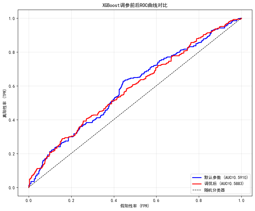

7. XGBoost vs 其他模型对比

print("="*60)
print("多模型性能对比")
print("="*60)

# 随机森林
rf = RandomForestClassifier(n_estimators=200, max_depth=10, random_state=42, n_jobs=-1)
rf.fit(X_train, y_train)
rf_proba = rf.predict_proba(X_test)[:, 1]

# GBDT
gbdt = GradientBoostingClassifier(n_estimators=200, learning_rate=0.1, max_depth=5, random_state=42)
gbdt.fit(X_train, y_train)
gbdt_proba = gbdt.predict_proba(X_test)[:, 1]

# LightGBM
lgb_model = lgb.LGBMClassifier(
    n_estimators=200,
    learning_rate=0.1,
    max_depth=5,
    random_state=42,
    n_jobs=-1,
    verbose=-1
)
lgb_model.fit(X_train, y_train)
lgb_proba = lgb_model.predict_proba(X_test)[:, 1]

# 收集结果
models_results = {
    '随机森林': rf_proba,
    'GBDT': gbdt_proba,
    'XGBoost默认': y_proba_default_final,
    'XGBoost调优': y_proba_best,
    'LightGBM': lgb_proba
}

# 打印性能表
print(f"\n{'模型':<15} {'准确率':<10} {'精确率':<10} {'召回率':<10} {'F1':<10} {'AUC':<10}")
print("-"*65)

for name, proba in models_results.items():
    pred = (proba > 0.5).astype(int)
    print(f"{name:<15} {accuracy_score(y_test, pred):<10.4f} "
          f"{precision_score(y_test, pred):<10.4f} {recall_score(y_test, pred):<10.4f} "
          f"{f1_score(y_test, pred):<10.4f} {roc_auc_score(y_test, proba):<10.4f}")

# ROC曲线综合对比
plt.figure(figsize=(12, 8))
colors = ['blue', 'green', 'orange', 'red', 'purple']

for (name, proba), color in zip(models_results.items(), colors):
    fpr, tpr, _ = roc_curve(y_test, proba)
    auc = roc_auc_score(y_test, proba)
    plt.plot(fpr, tpr, color=color, linewidth=2, label=f'{name} (AUC={auc:.4f})')

plt.plot([0, 1], [0, 1], 'k--', linewidth=1, label='随机分类器')
plt.xlabel('假阳性率 (FPR)')
plt.ylabel('真阳性率 (TPR)')
plt.title('多模型ROC曲线对比')
plt.legend(loc='lower right')
plt.grid(True, alpha=0.3)
plt.show()

============================================================
多模型性能对比
============================================================

模型              准确率        精确率        召回率        F1         AUC       
-----------------------------------------------------------------
随机森林            0.5421     0.5172     0.5600     0.5377     0.5797    
GBDT            0.5421     0.5174     0.5514     0.5339     0.5797    
XGBoost默认       0.5815     0.5553     0.6029     0.5781     0.5910    
XGBoost调优       0.5557     0.5296     0.5886     0.5575     0.5883    
LightGBM        0.5340     0.5092     0.5543     0.5308     0.5663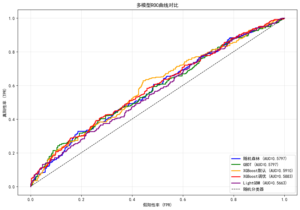    

8. LightGBM详解

8.1 LightGBM核心参数

┌─────────────────────────────────────────────────────────────────────────┐
│                        LightGBM核心参数                                 │
├─────────────────────────────────────────────────────────────────────────┤
│                                                                         │
│  num_leaves        : 每棵树的最大叶子数（默认31）                         │
│                     → 类似XGBoost的max_depth，但更灵活                   │
│                     → 典型值：15-63                                     │
│                                                                         │
│  max_depth         : 树的最大深度（默认-1，无限制）                       │
│                     → 配合num_leaves使用，防止过拟合                      │
│                                                                         │
│  learning_rate     : 学习率（默认0.1）                                  │
│                     → 典型值：0.01-0.3                                  │
│                                                                         │
│  n_estimators      : 树的数量（默认100）                                │
│                     → 配合早停使用                                       │
│                                                                         │
│  subsample         : 样本采样比例（默认1.0）                            │
│  colsample_bytree  : 特征采样比例（默认1.0）                            │
│                                                                         │
│  reg_alpha         : L1正则化（默认0）                                  │
│  reg_lambda        : L2正则化（默认0）                                  │
│                                                                         │
│  min_child_samples : 叶节点最小样本数（默认20）                          │
│  min_child_weight  : 叶节点最小权重和（默认0.001）                        │
│                                                                         │
└─────────────────────────────────────────────────────────────────────────┘

8.2 LightGBM训练与调参

def train_lightgbm_with_search(X_train, y_train, X_test, y_test):
    """训练并优化LightGBM"""
    
    # 基础LightGBM
    lgb_base = lgb.LGBMClassifier(
        n_estimators=200,
        learning_rate=0.1,
        num_leaves=31,
        random_state=42,
        n_jobs=-1,
        verbose=-1
    )
    
    # 参数网格
    param_grid = {
        'num_leaves': [15, 31, 63],
        'learning_rate': [0.05, 0.1, 0.2],
        'max_depth': [5, 7, 10, -1],
        'subsample': [0.6, 0.8, 1.0],
        'colsample_bytree': [0.6, 0.8, 1.0]
    }
    
    tscv = TimeSeriesSplit(n_splits=3)
    
    random_search = RandomizedSearchCV(
        lgb_base, param_grid,
        n_iter=20,
        cv=tscv,
        scoring='roc_auc',
        n_jobs=-1,
        random_state=42,
        verbose=1
    )
    
    print("LightGBM随机搜索...")
    start_time = time.time()
    random_search.fit(X_train, y_train)
    elapsed = time.time() - start_time
    
    print(f"\n搜索完成，耗时: {elapsed:.2f}秒")
    print(f"最佳参数: {random_search.best_params_}")
    print(f"最佳CV AUC: {random_search.best_score_:.4f}")
    
    best_lgb = random_search.best_estimator_
    y_proba_lgb = best_lgb.predict_proba(X_test)[:, 1]
    
    print(f"\n测试集AUC: {roc_auc_score(y_test, y_proba_lgb):.4f}")
    
    return best_lgb

# 训练LightGBM
best_lgb = train_lightgbm_with_search(X_train, y_train, X_test, y_test)

LightGBM随机搜索...
Fitting 3 folds for each of 20 candidates, totalling 60 fits

搜索完成，耗时: 6.47秒
最佳参数: {'subsample': 0.6, 'num_leaves': 31, 'max_depth': 5, 'learning_rate': 0.05, 'colsample_bytree': 1.0}
最佳CV AUC: 0.5073

测试集AUC: 0.5790

9. 特征重要性深入分析

9.1 XGBoost特征重要性类型

XGBoost提供多种特征重要性计算方式：

1. weight (默认): 特征被用作分裂点的次数
2. gain: 特征带来的平均增益（信息量）
3. cover: 特征覆盖的样本数
4. total_gain: 特征带来的总增益
5. total_cover: 特征覆盖的总样本数

建议：

• 分类任务：使用 gain 或 weight
• 特征选择：使用 total_gain

# 演示不同重要性类型
importance_types = ['weight', 'gain', 'cover']

fig, axes = plt.subplots(1, 3, figsize=(15, 5))

for idx, imp_type in enumerate(importance_types):
    # 获取特征重要性
    importance_dict = xgb_default_final.get_booster().get_score(importance_type=imp_type)
    
    # 转换为DataFrame
    if importance_dict:
        imp_df = pd.DataFrame({
            'feature': list(importance_dict.keys()),
            'importance': list(importance_dict.values())
        }).sort_values('importance', ascending=False)
        
        axes[idx].barh(imp_df['feature'][:8], imp_df['importance'][:8])
        axes[idx].set_title(f'{imp_type} 类型重要性')
        axes[idx].set_xlabel('重要性')
        axes[idx].grid(True, alpha=0.3)
    else:
        axes[idx].text(0.5, 0.5, f'{imp_type}类型无数据', ha='center', transform=axes[idx].transAxes)
        axes[idx].set_title(f'{imp_type} 类型')

plt.tight_layout()
plt.show()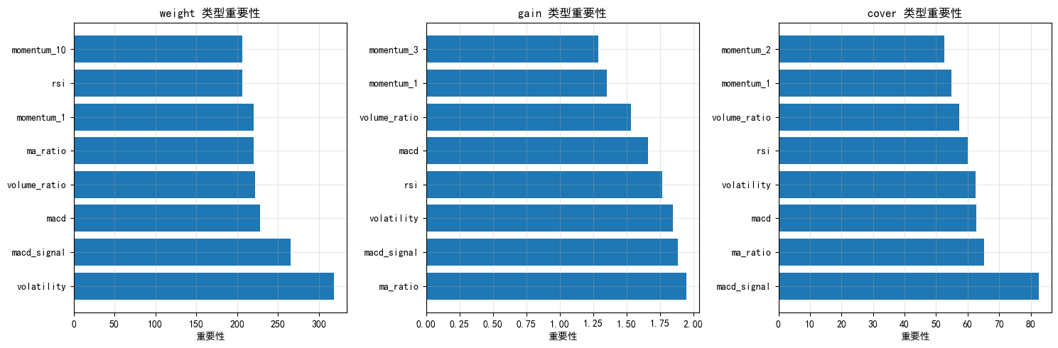

10. 今日总结

1. XGBoost核心原理：

   • 二阶泰勒展开（比GBDT更精确）
   • 内置正则化（gamma、lambda、alpha）
   • 并行计算支持

2. LightGBM核心创新：

   • 直方图算法（速度↑，内存↓）
   • Leaf-wise生长策略
   • GOSS采样（减少样本）
   • EFB特征捆绑

3. 调参策略：

   • 第一阶段：调树结构（max_depth, min_child_weight）
   • 第二阶段：调学习率与树数量
   • 第三阶段：调正则化参数（gamma, lambda, subsample）
   • 使用早停自动确定最佳树数量

4. 模型对比：

   • 随机森林：方差低，对异常值鲁棒
   • GBDT：传统Boosting
   • XGBoost：精度高，正则化强
   • LightGBM：速度快，内存低

5. 量化交易应用：

   • XGBoost/LightGBM是目前量化选股的主流工具
   • 融合模型（Stacking）可进一步提升效果
   • 使用时间序列交叉验证避免前视偏差

6. 扩展作业

   • 作业1：尝试不同的特征重要性类型（gain/weight/cover），对比特征排序差异
   • 作业2：实现XGBoost和LightGBM的Stacking融合模型
   • 作业3：在实际股票数据上测试XGBoost策略（使用yfinance获取数据）
   • 作业4：使用早停训练LightGBM，并绘制训练过程损失曲线
   • 作业5：调整XGBoost的eval_metric为不同指标（auc、logloss、error），观察差异

7. 量化思考

   • XGBoost/LightGBM是目前量化选股的主流工具
   • 在大数据集上，LightGBM速度优势明显
   • 小数据集上，XGBoost可能表现更好
   • 结合早停和交叉验证可以有效防止过拟合
   • 可考虑多模型融合（Stacking）进一步提升效果