深度学习(6)softmax回归、损失函数、分类

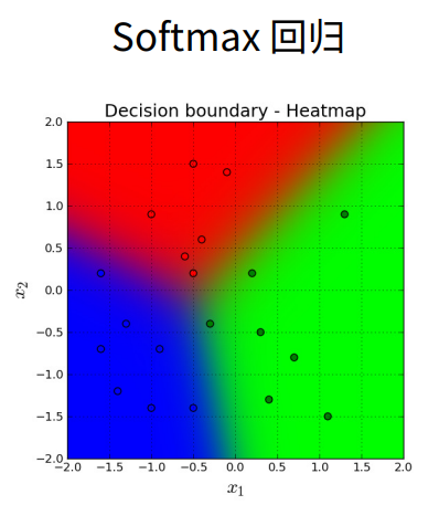
1. Softmax回归

① Softmax回归虽然它的名字是回归，其实它是一个分类问题。

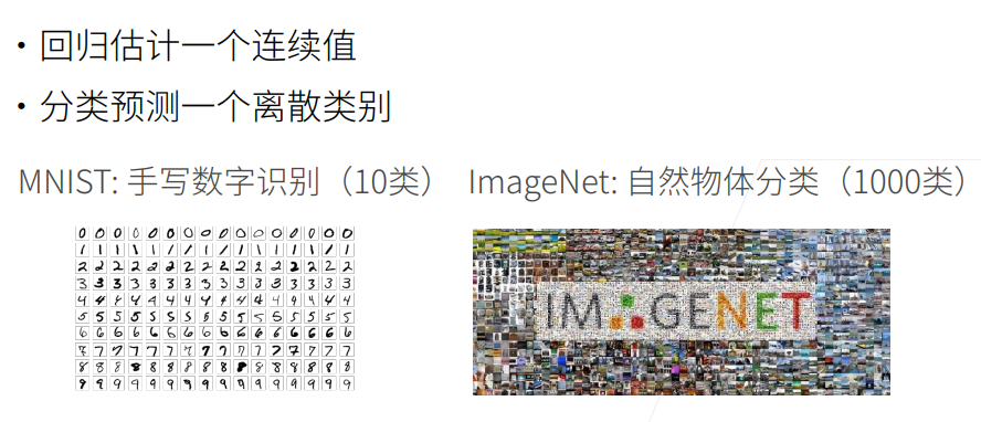
2. 回归VS分类

3. Kaggle分类问题

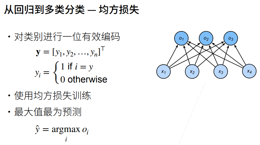
4. 回归到分类

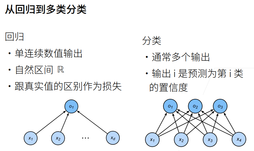
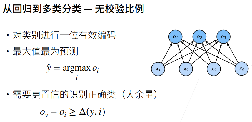
分类时，我们不关系实际的值，我们关心的是能不能对正确的类的置信度特别大，比如将正确的类的置信度写成Oy,那么要远远大于其他非正确类的Oy，也就是二者相减大于一个阈值。
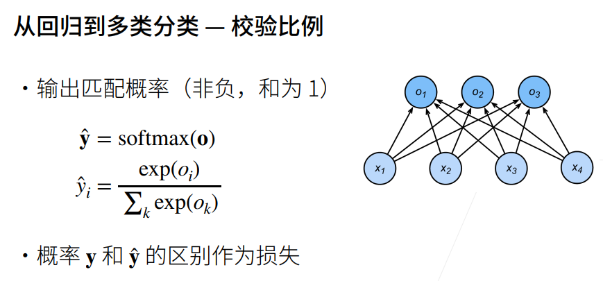
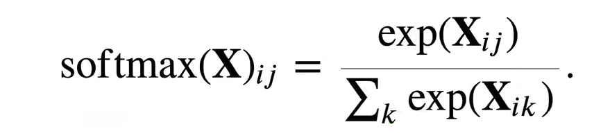
我们希望我们的输出是一个概率，就使用softmax；

指数运算的好处就是，不管什么值，都可以变成非负
y^i=(Oi做指数运算)/(所有的Ok做指数相加)

这样y_hat就是一个概率了，

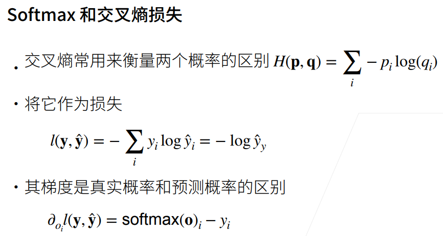
5. 交叉熵损失

6. 总结

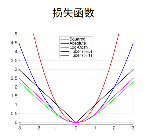
7. 损失函数

① 三个常用的损失函数 L2 loss、L1 loss、Huber's Robust loss。

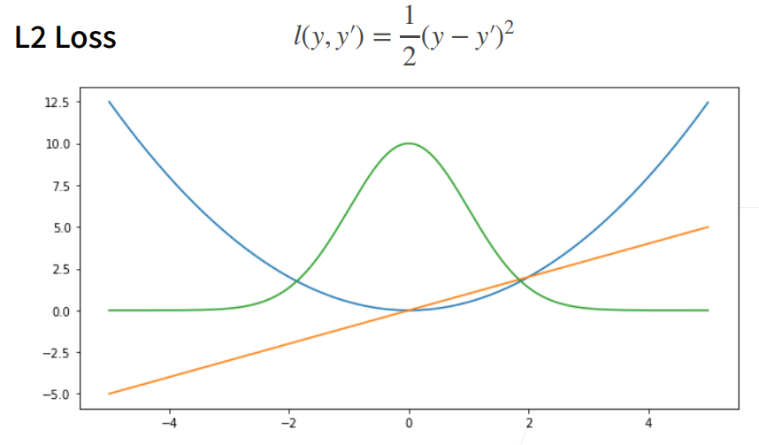
8. L2 Loss[均方损失]

① 蓝色曲线为当y=0时，变换y'所获得的曲线。

② 绿色曲线为当y=0时，变换y'所获得的曲线的似然函数，即，似然函数呈高斯分布。最小化损失函数就是最大化似然函数。

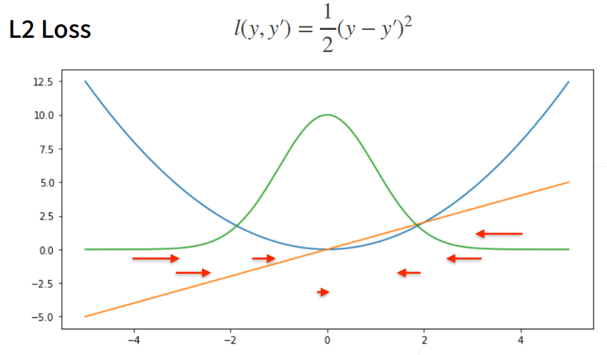
③ 橙色曲线为损失函数的梯度，梯度是一次函数，所以穿过原点。

④ 当预测值y'跟真实值y隔的比较远的时候，(真实值y为0，预测值就是下面的曲线里的x轴)，梯度比较大，所以参数更新比较多。

⑤ 随着预测值靠近真实值时，梯度越来越小，参数的更新越来越小。

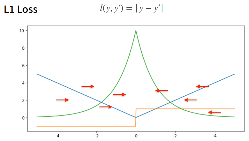
9. L1 Loss[绝对值损失函数]

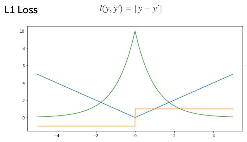
① 相对L2 loss，L1 loss的梯度就是距离原点时，梯度也不是特别大，权重的更新也不是特别大。会带来很多稳定性的好处。

② 他的缺点是在零点处不可导，并在零点处左右有±1的变化，这个不平滑性导致预测值与真实值靠的比较近的时候，优化到末期的时候，可能会不那么稳定。

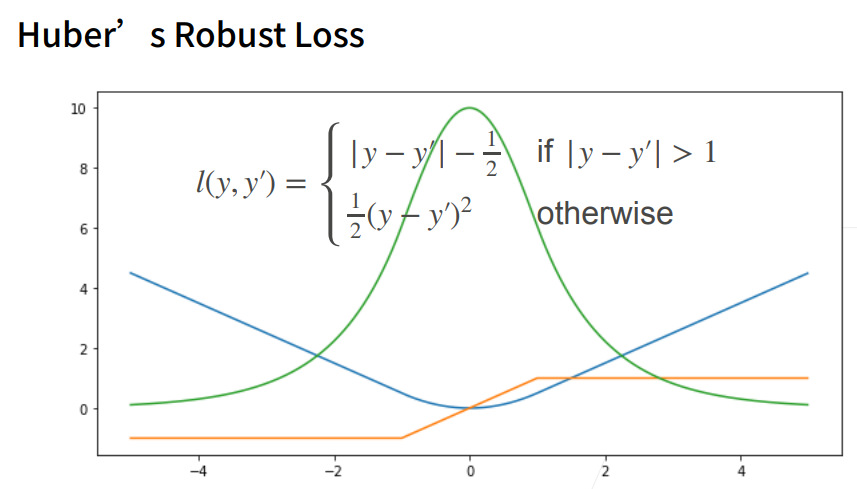
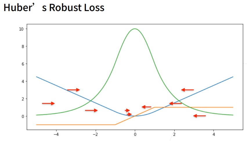
10. Huber's Robust Loss

① 结合L1 loss 和L2 loss损失。

当预测值和真实值差的比较大的时候[绝对值>1时],我是一个绝对值误差；

当预测值和真实值靠的比较近的时候[绝对值<=1时]，就是平方误差

这样保证优化是比较平滑的，

1. 图像分类数据集

① MINIST数据集是图像分类中广泛使用的数据集之一，但作为基准数据集过于简单。

② 下面将使用类似但更复杂的Fashion-MNIST数据集。

1.1 显示图片

%matplotlib inline
import torch
import torchvision #对计算机视觉模型实现的库
from torch.utils import data
from torchvision import transforms
from d2l import torch as d2l

# SVG是一种无损格式 -- 意味着它在压缩时不会丢失任何数据，可以呈现无限数量的颜色。
# SVG最常用于网络上的图形、徽标可供其他高分辨率屏幕上查看。
d2l.use_svg_display() # 使用svg来显示图片，这样清晰度高一些。
help(d2l.use_svg_display)
Help on function use_svg_display in module d2l.torch:

use_svg_display()
    Use the svg format to display a plot in Jupyter.

库/模块	作用
%matplotlib inline	Jupyter魔法命令，让matplotlib绘制的图形直接显示在网页中（不弹出新窗口）
torch	PyTorch深度学习框架，提供张量计算、自动求导、神经网络模块等核心功能
torchvision	PyTorch的计算机视觉扩展库，提供经典数据集（如CIFAR、MNIST）、预训练模型、图像变换工具
torch.utils.data	数据加载工具，提供Dataset（数据集类）和DataLoader（批量数据加载器）
torchvision.transforms	图像预处理工具，支持裁剪、缩放、归一化、转张量等常见数据增强操作
d2l (torch版)	《动手学深度学习》配套工具库，封装了绘图简化、数据加载、训练循环、天气等辅助函数
d2l.use_svg_display()	d2l库中的函数，设置matplotlib使用SVG矢量格式显示图形（缩放不失真，适合高清展示）

SVG vs 普通图片

特性	SVG	PNG/JPG
缩放	无限放大不失真	放大变模糊
文件大小	较小（图形简单时）	较大
适用场景	图表、logo、矢量图	照片、复杂图像

1.2 数据集下载

通过框架中的内置函数将Fashion-MNIST数据集下载并读取到内存中

%matplotlib inline
import torch
import torchvision
from torch.utils import data
from torchvision import transforms
from d2l import torch as d2l

d2l.use_svg_display()

# 通过ToTensor实例将图像数据从PIL类型变换成32位浮点数格式
# 并除以255使得所有像素的数值均在0到1之间
trans = transforms.ToTensor()
#训练集
mnist_train = torchvision.datasets.FashionMNIST(
    root="G:/database/01_DataSet_FashionMNIST",  # 数据集将下载到这里
    train=True,   # True=训练集，False=测试集
    transform=trans,  # 应用上面定义的预处理
    download=True    # 如果本地没有就自动下载
)
#测试集
mnist_test = torchvision.datasets.FashionMNIST(
    root="G:/database/01_DataSet_FashionMNIST",
    train=False,
    transform=trans,
    download=True
)           
print(len(mnist_train)) # 训练数据集长度
print(len(mnist_test))  # 测试数据集长度

print(mnist_train[0][0].shape) # 黑白图片，所以channel为1。
print(mnist_train[0][1]) # [0][0]表示第一个样本的图片信息，[0][1]表示该样本对应的标签值

60000
10000
torch.Size([1, 28, 28])
9

1.3 可视化数据集

第一个函数：把数字标签（0-9）转换成对应的服装名称

第二个函数：显示图片网格：

• imgs：要显示的图片列表

• num_rows：网格行数

• num_cols：网格列数

• titles：每张图片的标题

• scale：图片缩放比例

第1步：创建画布；

第2步：将二维数组展平成一维；

第3步：在每张子图上显示图片

获取数据

# DataLoader：批量加载数据
loader = data.DataLoader(mnist_train, batch_size=18)
# 每次加载18张图片和对应的标签

# iter()：创建迭代器
iterator = iter(loader)

# next()：取一批数据
X, y = next(iterator)
# X: 18张图片，形状 [18, 1, 28, 28] (批大小, 通道, 高, 宽)
# y: 18个标签，形状 [18]

显示图片

• X.reshape(18,28,28)：去掉通道维度 [18,1,28,28] → [18,28,28]

• 2, 9：2行9列，总共显示18张图

• titles=get_fashion_mnist_labels(y)：把数字标签转成文字作为标题

%matplotlib inline
import torch
import torchvision
from torch.utils import data
from torchvision import transforms
from d2l import torch as d2l

d2l.use_svg_display()

# 通过ToTensor实例将图像数据从PIL类型变换成32位浮点数格式
# 并除以255使得所有像素的数值均在0到1之间
trans = transforms.ToTensor()
mnist_train = torchvision.datasets.FashionMNIST(root="01_data/01_DataSet_FashionMNIST",train=True,transform=trans,download=True)
mnist_test = torchvision.datasets.FashionMNIST(root="01_data/01_DataSet_FashionMNIST",train=False,transform=trans,download=True)            

def get_fashion_mnist_labels(labels):
    """返回Fashion-MNIST数据集的文本标签"""
    text_labels = ['t-shirt','trouser','pullover','dress','coat',
                   'sandal','shirt','sneaker','bag','ankle boot']
    return [text_labels[int(i)] for i in labels]

def show_images(imgs, num_rows, num_cols, titles=None, scale=1.5):
    """Plot a list of images."""
    figsize = (num_cols * scale, num_rows * scale) # 传进来的图像尺寸，scale 为放缩比例因子
    _, axes = d2l.plt.subplots(num_rows,num_cols,figsize=figsize)
# subplots创建2行9列的子图网格，返回(图形对象, 坐标轴数组)
    print(_)
    print(axes) # axes 为构建的两行九列的画布
#将二维数组展平成一维
    axes = axes.flatten()
    print(axes) # axes 变成一维数据
    for i,(ax,img) in enumerate(zip(axes,imgs)):
        if(i<1):
            print("i:",i)
            print("ax,img:",ax,img)
        if torch.is_tensor(img):
            # 图片张量
            ax.imshow(img.numpy())  # 张量→numpy数组→显示
            ax.set_title(titles[i])
        else:
            # PIL图片
            ax.imshow(img) # 直接显示PIL图片
            
X, y = next(iter(data.DataLoader(mnist_train,batch_size=18))) # X，y 为仅抽取一次的18个样本的图片、以及对应的标签值
show_images(X.reshape(18,28,28),2,9,titles=get_fashion_mnist_labels(y))

Figure(972x216)
[[<AxesSubplot:> <AxesSubplot:> <AxesSubplot:> <AxesSubplot:>
  <AxesSubplot:> <AxesSubplot:> <AxesSubplot:> <AxesSubplot:>
  <AxesSubplot:>]
 [<AxesSubplot:> <AxesSubplot:> <AxesSubplot:> <AxesSubplot:>
  <AxesSubplot:> <AxesSubplot:> <AxesSubplot:> <AxesSubplot:>
  <AxesSubplot:>]]
[<AxesSubplot:> <AxesSubplot:> <AxesSubplot:> <AxesSubplot:>
 <AxesSubplot:> <AxesSubplot:> <AxesSubplot:> <AxesSubplot:>
 <AxesSubplot:> <AxesSubplot:> <AxesSubplot:> <AxesSubplot:>
 <AxesSubplot:> <AxesSubplot:> <AxesSubplot:> <AxesSubplot:>
 <AxesSubplot:> <AxesSubplot:>]
i: 0
ax,img: AxesSubplot(0.125,0.536818;0.0731132x0.343182) tensor([[0.0000, 0.0000, 0.0000, 0.0000, 0.0000, 0.0000, 0.0000, 0.0000, 0.0000,
         0.0000, 0.0000, 0.0000, 0.0000, 0.0000, 0.0000, 0.0000, 0.0000, 0.0000,
         0.0000, 0.0000, 0.0000, 0.0000, 0.0000, 0.0000, 0.0000, 0.0000, 0.0000,
         0.0000],
        [0.0000, 0.0000, 0.0000, 0.0000, 0.0000, 0.0000, 0.0000, 0.0000, 0.0000,
         0.0000, 0.0000, 0.0000, 0.0000, 0.0000, 0.0000, 0.0000, 0.0000, 0.0000,
         0.0000, 0.0000, 0.0000, 0.0000, 0.0000, 0.0000, 0.0000, 0.0000, 0.0000,
         0.0000],
        [0.0000, 0.0000, 0.0000, 0.0000, 0.0000, 0.0000, 0.0000, 0.0000, 0.0000,
         0.0000, 0.0000, 0.0000, 0.0000, 0.0000, 0.0000, 0.0000, 0.0000, 0.0000,
         0.0000, 0.0000, 0.0000, 0.0000, 0.0000, 0.0000, 0.0000, 0.0000, 0.0000,
         0.0000],
        [0.0000, 0.0000, 0.0000, 0.0000, 0.0000, 0.0000, 0.0000, 0.0000, 0.0000,
         0.0000, 0.0000, 0.0000, 0.0039, 0.0000, 0.0000, 0.0510, 0.2863, 0.0000,
         0.0000, 0.0039, 0.0157, 0.0000, 0.0000, 0.0000, 0.0000, 0.0039, 0.0039,
         0.0000],
        [0.0000, 0.0000, 0.0000, 0.0000, 0.0000, 0.0000, 0.0000, 0.0000, 0.0000,
         0.0000, 0.0000, 0.0000, 0.0118, 0.0000, 0.1412, 0.5333, 0.4980, 0.2431,
         0.2118, 0.0000, 0.0000, 0.0000, 0.0039, 0.0118, 0.0157, 0.0000, 0.0000,
         0.0118],
        [0.0000, 0.0000, 0.0000, 0.0000, 0.0000, 0.0000, 0.0000, 0.0000, 0.0000,
         0.0000, 0.0000, 0.0000, 0.0235, 0.0000, 0.4000, 0.8000, 0.6902, 0.5255,
         0.5647, 0.4824, 0.0902, 0.0000, 0.0000, 0.0000, 0.0000, 0.0471, 0.0392,
         0.0000],
        [0.0000, 0.0000, 0.0000, 0.0000, 0.0000, 0.0000, 0.0000, 0.0000, 0.0000,
         0.0000, 0.0000, 0.0000, 0.0000, 0.0000, 0.6078, 0.9255, 0.8118, 0.6980,
         0.4196, 0.6118, 0.6314, 0.4275, 0.2510, 0.0902, 0.3020, 0.5098, 0.2824,
         0.0588],
        [0.0000, 0.0000, 0.0000, 0.0000, 0.0000, 0.0000, 0.0000, 0.0000, 0.0000,
         0.0000, 0.0000, 0.0039, 0.0000, 0.2706, 0.8118, 0.8745, 0.8549, 0.8471,
         0.8471, 0.6392, 0.4980, 0.4745, 0.4784, 0.5725, 0.5529, 0.3451, 0.6745,
         0.2588],
        [0.0000, 0.0000, 0.0000, 0.0000, 0.0000, 0.0000, 0.0000, 0.0000, 0.0000,
         0.0039, 0.0039, 0.0039, 0.0000, 0.7843, 0.9098, 0.9098, 0.9137, 0.8980,
         0.8745, 0.8745, 0.8431, 0.8353, 0.6431, 0.4980, 0.4824, 0.7686, 0.8980,
         0.0000],
        [0.0000, 0.0000, 0.0000, 0.0000, 0.0000, 0.0000, 0.0000, 0.0000, 0.0000,
         0.0000, 0.0000, 0.0000, 0.0000, 0.7176, 0.8824, 0.8471, 0.8745, 0.8941,
         0.9216, 0.8902, 0.8784, 0.8706, 0.8784, 0.8667, 0.8745, 0.9608, 0.6784,
         0.0000],
        [0.0000, 0.0000, 0.0000, 0.0000, 0.0000, 0.0000, 0.0000, 0.0000, 0.0000,
         0.0000, 0.0000, 0.0000, 0.0000, 0.7569, 0.8941, 0.8549, 0.8353, 0.7765,
         0.7059, 0.8314, 0.8235, 0.8275, 0.8353, 0.8745, 0.8627, 0.9529, 0.7922,
         0.0000],
        [0.0000, 0.0000, 0.0000, 0.0000, 0.0000, 0.0000, 0.0000, 0.0000, 0.0000,
         0.0039, 0.0118, 0.0000, 0.0471, 0.8588, 0.8627, 0.8314, 0.8549, 0.7529,
         0.6627, 0.8902, 0.8157, 0.8549, 0.8784, 0.8314, 0.8863, 0.7725, 0.8196,
         0.2039],
        [0.0000, 0.0000, 0.0000, 0.0000, 0.0000, 0.0000, 0.0000, 0.0000, 0.0000,
         0.0000, 0.0235, 0.0000, 0.3882, 0.9569, 0.8706, 0.8627, 0.8549, 0.7961,
         0.7765, 0.8667, 0.8431, 0.8353, 0.8706, 0.8627, 0.9608, 0.4667, 0.6549,
         0.2196],
        [0.0000, 0.0000, 0.0000, 0.0000, 0.0000, 0.0000, 0.0000, 0.0000, 0.0000,
         0.0157, 0.0000, 0.0000, 0.2157, 0.9255, 0.8941, 0.9020, 0.8941, 0.9412,
         0.9098, 0.8353, 0.8549, 0.8745, 0.9176, 0.8510, 0.8510, 0.8196, 0.3608,
         0.0000],
        [0.0000, 0.0000, 0.0039, 0.0157, 0.0235, 0.0275, 0.0078, 0.0000, 0.0000,
         0.0000, 0.0000, 0.0000, 0.9294, 0.8863, 0.8510, 0.8745, 0.8706, 0.8588,
         0.8706, 0.8667, 0.8471, 0.8745, 0.8980, 0.8431, 0.8549, 1.0000, 0.3020,
         0.0000],
        [0.0000, 0.0118, 0.0000, 0.0000, 0.0000, 0.0000, 0.0000, 0.0000, 0.0000,
         0.2431, 0.5686, 0.8000, 0.8941, 0.8118, 0.8353, 0.8667, 0.8549, 0.8157,
         0.8275, 0.8549, 0.8784, 0.8745, 0.8588, 0.8431, 0.8784, 0.9569, 0.6235,
         0.0000],
        [0.0000, 0.0000, 0.0000, 0.0000, 0.0706, 0.1725, 0.3216, 0.4196, 0.7412,
         0.8941, 0.8627, 0.8706, 0.8510, 0.8863, 0.7843, 0.8039, 0.8275, 0.9020,
         0.8784, 0.9176, 0.6902, 0.7373, 0.9804, 0.9725, 0.9137, 0.9333, 0.8431,
         0.0000],
        [0.0000, 0.2235, 0.7333, 0.8157, 0.8784, 0.8667, 0.8784, 0.8157, 0.8000,
         0.8392, 0.8157, 0.8196, 0.7843, 0.6235, 0.9608, 0.7569, 0.8078, 0.8745,
         1.0000, 1.0000, 0.8667, 0.9176, 0.8667, 0.8275, 0.8627, 0.9098, 0.9647,
         0.0000],
        [0.0118, 0.7922, 0.8941, 0.8784, 0.8667, 0.8275, 0.8275, 0.8392, 0.8039,
         0.8039, 0.8039, 0.8627, 0.9412, 0.3137, 0.5882, 1.0000, 0.8980, 0.8667,
         0.7373, 0.6039, 0.7490, 0.8235, 0.8000, 0.8196, 0.8706, 0.8941, 0.8824,
         0.0000],
        [0.3843, 0.9137, 0.7765, 0.8235, 0.8706, 0.8980, 0.8980, 0.9176, 0.9765,
         0.8627, 0.7608, 0.8431, 0.8510, 0.9451, 0.2549, 0.2863, 0.4157, 0.4588,
         0.6588, 0.8588, 0.8667, 0.8431, 0.8510, 0.8745, 0.8745, 0.8784, 0.8980,
         0.1137],
        [0.2941, 0.8000, 0.8314, 0.8000, 0.7569, 0.8039, 0.8275, 0.8824, 0.8471,
         0.7255, 0.7725, 0.8078, 0.7765, 0.8353, 0.9412, 0.7647, 0.8902, 0.9608,
         0.9373, 0.8745, 0.8549, 0.8314, 0.8196, 0.8706, 0.8627, 0.8667, 0.9020,
         0.2627],
        [0.1882, 0.7961, 0.7176, 0.7608, 0.8353, 0.7725, 0.7255, 0.7451, 0.7608,
         0.7529, 0.7922, 0.8392, 0.8588, 0.8667, 0.8627, 0.9255, 0.8824, 0.8471,
         0.7804, 0.8078, 0.7294, 0.7098, 0.6941, 0.6745, 0.7098, 0.8039, 0.8078,
         0.4510],
        [0.0000, 0.4784, 0.8588, 0.7569, 0.7020, 0.6706, 0.7176, 0.7686, 0.8000,
         0.8235, 0.8353, 0.8118, 0.8275, 0.8235, 0.7843, 0.7686, 0.7608, 0.7490,
         0.7647, 0.7490, 0.7765, 0.7529, 0.6902, 0.6118, 0.6549, 0.6941, 0.8235,
         0.3608],
        [0.0000, 0.0000, 0.2902, 0.7412, 0.8314, 0.7490, 0.6863, 0.6745, 0.6863,
         0.7098, 0.7255, 0.7373, 0.7412, 0.7373, 0.7569, 0.7765, 0.8000, 0.8196,
         0.8235, 0.8235, 0.8275, 0.7373, 0.7373, 0.7608, 0.7529, 0.8471, 0.6667,
         0.0000],
        [0.0078, 0.0000, 0.0000, 0.0000, 0.2588, 0.7843, 0.8706, 0.9294, 0.9373,
         0.9490, 0.9647, 0.9529, 0.9569, 0.8667, 0.8627, 0.7569, 0.7490, 0.7020,
         0.7137, 0.7137, 0.7098, 0.6902, 0.6510, 0.6588, 0.3882, 0.2275, 0.0000,
         0.0000],
        [0.0000, 0.0000, 0.0000, 0.0000, 0.0000, 0.0000, 0.0000, 0.1569, 0.2392,
         0.1725, 0.2824, 0.1608, 0.1373, 0.0000, 0.0000, 0.0000, 0.0000, 0.0000,
         0.0000, 0.0000, 0.0000, 0.0000, 0.0000, 0.0000, 0.0000, 0.0000, 0.0000,
         0.0000],
        [0.0000, 0.0000, 0.0000, 0.0000, 0.0000, 0.0000, 0.0000, 0.0000, 0.0000,
         0.0000, 0.0000, 0.0000, 0.0000, 0.0000, 0.0000, 0.0000, 0.0000, 0.0000,
         0.0000, 0.0000, 0.0000, 0.0000, 0.0000, 0.0000, 0.0000, 0.0000, 0.0000,
         0.0000],
        [0.0000, 0.0000, 0.0000, 0.0000, 0.0000, 0.0000, 0.0000, 0.0000, 0.0000,
         0.0000, 0.0000, 0.0000, 0.0000, 0.0000, 0.0000, 0.0000, 0.0000, 0.0000,
         0.0000, 0.0000, 0.0000, 0.0000, 0.0000, 0.0000, 0.0000, 0.0000, 0.0000,
         0.0000]])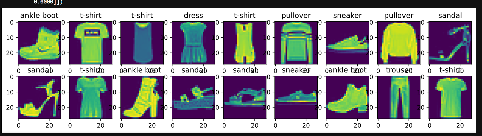

1.4 小批量数据集

%matplotlib inline
import torch
import torchvision
from torch.utils import data
from torchvision import transforms
from d2l import torch as d2l

d2l.use_svg_display()

# 通过ToTensor实例将图像数据从PIL类型变换成32位浮点数格式
# 并除以255使得所有像素的数值均在0到1之间
trans = transforms.ToTensor()
mnist_train = torchvision.datasets.FashionMNIST(root="01_data/01_DataSet_FashionMNIST",train=True,transform=trans,download=True)
mnist_test = torchvision.datasets.FashionMNIST(root="01_data/01_DataSet_FashionMNIST",train=False,transform=trans,download=True)            

def get_fashion_mnist_labels(labels):
    """返回Fashion-MNIST数据集的文本标签"""
    text_labels = ['t-shirt','trouser','pullover','dress','coat',
                   'sandal','shirt','sneaker','bag','ankle boot']
    return [text_labels[int(i)] for i in labels]

def show_images(imgs, num_rows, num_cols, titles=None, scale=1.5):
    """Plot a list of images."""
    figsize = (num_cols * scale, num_rows * scale) # 传进来的图像尺寸，scale 为放缩比例因子
    _, axes = d2l.plt.subplots(num_rows,num_cols,figsize=figsize)
    print(_)
    print(axes) # axes 为构建的两行九列的画布
    axes = axes.flatten()
    print(axes) # axes 变成一维数据
    for i,(ax,img) in enumerate(zip(axes,imgs)):
        if torch.is_tensor(img):
            # 图片张量
            ax.imshow(img.numpy())
            ax.set_title(titles[i])
        else:
            # PIL图片
            ax.imshow(img)
            
X, y = next(iter(data.DataLoader(mnist_train,batch_size=18))) # X，y 为仅抽取一次的18个样本的图片、以及对应的标签值
show_images(X.reshape(18,28,28),2,9,titles=get_fashion_mnist_labels(y))

#设置批量大小；每次从数据集中取 256张图片 进行处理
batch_size = 256

# 设置数据加载进程数
def get_dataloader_workers():
    """使用4个进程来读取的数据"""
    return 4   #多进程可以加快数据读取速度（特别是数据量大或图片需要预处理时）

# 创建数据加载器    
train_iter = data.DataLoader(
    mnist_train,           # 数据集
    batch_size,            # 256，批量大小
    shuffle=True,          # 打乱顺序，避免模型记住数据顺序
    num_workers=get_dataloader_workers()  # 4个进程
)

#计时测试
timer = d2l.Timer() # 计时器对象实例化，开始计时
for X,y in train_iter:  # 遍历一个batch_size数据的时间
    continue        # 什么都不做，只是读取数据
f'{timer.stop():.2f}sec' # 计时器停止时，返回停止与开始的时间间隔事件

Figure(972x216)
[[<AxesSubplot:> <AxesSubplot:> <AxesSubplot:> <AxesSubplot:>
  <AxesSubplot:> <AxesSubplot:> <AxesSubplot:> <AxesSubplot:>
  <AxesSubplot:>]
 [<AxesSubplot:> <AxesSubplot:> <AxesSubplot:> <AxesSubplot:>
  <AxesSubplot:> <AxesSubplot:> <AxesSubplot:> <AxesSubplot:>
  <AxesSubplot:>]]
[<AxesSubplot:> <AxesSubplot:> <AxesSubplot:> <AxesSubplot:>
 <AxesSubplot:> <AxesSubplot:> <AxesSubplot:> <AxesSubplot:>
 <AxesSubplot:> <AxesSubplot:> <AxesSubplot:> <AxesSubplot:>
 <AxesSubplot:> <AxesSubplot:> <AxesSubplot:> <AxesSubplot:>
 <AxesSubplot:> <AxesSubplot:>]

'1.62sec'

会显示 d2l 库中 Timer 类的文档说明

help(d2l.Timer)

Help on class Timer in module d2l.torch:

class Timer(builtins.object)
 |  Record multiple running times.
 |  
 |  Methods defined here:
 |  
 |  __init__(self)
 |      Initialize self.  See help(type(self)) for accurate signature.
 |  
 |  avg(self)
 |      Return the average time.
 |  
 |  cumsum(self)
 |      Return the accumulated time.
 |  
 |  start(self)
 |      Start the timer.
 |  
 |  stop(self)
 |      Stop the timer and record the time in a list.
 |  
 |  sum(self)
 |      Return the sum of time.
 |  
 |  ----------------------------------------------------------------------
 |  Data descriptors defined here:
 |  
 |  __dict__
 |      dictionary for instance variables (if defined)
 |  
 |  __weakref__
 |      list of weak references to the object (if defined)

class Timer(d2l.torch.Timer)
| 记录多次运行时间的类。
|
| 方法：
| init(self)
| 初始化一个计时器，记录开始时间。
|
| start(self)
| 启动计时器，记录开始时间。
|
| stop(self)
| 停止计时器，返回经过的时间间隔（秒）。
|
| reset(self)
| 重置计时器，归零并重新开始。
|
| times(self)
| 返回所有记录的时间列表。
|
| avg(self)
| 返回平均耗时。
|
| sum(self)
| 返回总耗时。
|
| cumsum(self)
| 返回累计时间列表。
|
| enter(self)
| 支持上下文管理器（with语句）。
|
| exit(self, *args)
| 退出上下文管理器时自动停止。

**Example:
timer = d2l.Timer()

执行某个操作

print(f'{timer.stop():.2f} sec')

或使用上下文管理器

with d2l.Timer() as timer:

执行操作

pass
print(f'{timer.stop():.2f} sec')**

1.5 加载数据集

%matplotlib inline
import torch
import torchvision
from torch.utils import data
from torchvision import transforms
from d2l import torch as d2l

d2l.use_svg_display()

# 通过ToTensor实例将图像数据从PIL类型变换成32位浮点数格式
# 并除以255使得所有像素的数值均在0到1之间
trans = transforms.ToTensor()
mnist_train = torchvision.datasets.FashionMNIST(root="01_data/01_DataSet_FashionMNIST",train=True,transform=trans,download=True)
mnist_test = torchvision.datasets.FashionMNIST(root="01_data/01_DataSet_FashionMNIST",train=False,transform=trans,download=True)            

def get_fashion_mnist_labels(labels):
    """返回Fashion-MNIST数据集的文本标签"""
    text_labels = ['t-shirt','trouser','pullover','dress','coat',
                   'sandal','shirt','sneaker','bag','ankle boot']
    return [text_labels[int(i)] for i in labels]

def show_images(imgs, num_rows, num_cols, titles=None, scale=1.5):
    """Plot a list of images."""
    figsize = (num_cols * scale, num_rows * scale) # 传进来的图像尺寸，scale 为放缩比例因子
    _, axes = d2l.plt.subplots(num_rows,num_cols,figsize=figsize)
    print(_)
    print(axes) # axes 为构建的两行九列的画布
    axes = axes.flatten()
    print(axes) # axes 变成一维数据
    for i,(ax,img) in enumerate(zip(axes,imgs)):
        if torch.is_tensor(img):
            # 图片张量
            ax.imshow(img.numpy())
            ax.set_title(titles[i])
        else:
            # PIL图片
            ax.imshow(img)
            
X, y = next(iter(data.DataLoader(mnist_train,batch_size=18))) # X，y 为仅抽取一次的18个样本的图片、以及对应的标签值
show_images(X.reshape(18,28,28),2,9,titles=get_fashion_mnist_labels(y))

batch_size = 256
def get_dataloader_workers():
    """使用4个进程来读取的数据"""
    return 4

train_iter = data.DataLoader(mnist_train, batch_size, shuffle=True,
                            num_workers=get_dataloader_workers())

timer = d2l.Timer()
for X,y in train_iter:
    continue
f'{timer.stop():.2f}sec'  # 扫一边数据集的事件

def load_data_fashion_mnist(batch_size, resize=None):
    """下载Fashion-MNIST数据集，然后将其加载到内存中"""
    trans = [transforms.ToTensor()]  # 创建列表，包含一个预处理操作：将图片转成张量
    
    if resize:  # 如果有缩放需求，就在列表开头插入缩放操作
        trans.insert(0, transforms.Resize(resize))  # 如果有Resize参数传进来，就进行resize操作
    
    # 将多个预处理操作组合成一个流水线
    trans = transforms.Compose(trans)
    
    data_path = "G:/database/01_DataSet_FashionMNIST"  # 改成你的路径
    
    # 加载数据集 - 注意这里需要缩进
    mnist_train = torchvision.datasets.FashionMNIST(
        root=data_path,  # 使用 data_path，不是 root_data_path
        train=True,      # 训练集
        transform=trans, # 使用 trans，不是 transform_trans
        download=True
    )
    
    mnist_test = torchvision.datasets.FashionMNIST(
        root=data_path,   # 使用 data_path
        train=False,      # 测试集
        transform=trans,  # 使用 trans
        download=True
    )
    
    # 返回数据加载器 - 注意缩进与函数体对齐
    return (data.DataLoader(mnist_train, batch_size, shuffle=True, num_workers=get_dataloader_workers()),
            data.DataLoader(mnist_test, batch_size, shuffle=False, num_workers=get_dataloader_workers()))

函数定义

def load_data_fashion_mnist(batch_size, resize=None):
作用：定义一个函数，可以方便地加载Fashion-MNIST数据集
参数：
batch_size每批加载多少张图片（如256）
resize=None可选参数，如果提供就缩放图片尺寸

Figure(972x216)
[[<AxesSubplot:> <AxesSubplot:> <AxesSubplot:> <AxesSubplot:>
  <AxesSubplot:> <AxesSubplot:> <AxesSubplot:> <AxesSubplot:>
  <AxesSubplot:>]
 [<AxesSubplot:> <AxesSubplot:> <AxesSubplot:> <AxesSubplot:>
  <AxesSubplot:> <AxesSubplot:> <AxesSubplot:> <AxesSubplot:>
  <AxesSubplot:>]]
[<AxesSubplot:> <AxesSubplot:> <AxesSubplot:> <AxesSubplot:>
 <AxesSubplot:> <AxesSubplot:> <AxesSubplot:> <AxesSubplot:>
 <AxesSubplot:> <AxesSubplot:> <AxesSubplot:> <AxesSubplot:>
 <AxesSubplot:> <AxesSubplot:> <AxesSubplot:> <AxesSubplot:>
 <AxesSubplot:> <AxesSubplot:>]

2. Softmax回归（使用自定义）

① 就像从零开始实现线性回归一样，应该知道softmax的细节。

2.1 训练集、测试集抽取

import torch
from IPython import display
from d2l import torch as d2l

def load_data_fashion_mnist(batch_size, resize=None):
    """下载Fashion-MNIST数据集，然后将其加载到内存中"""
    trans = [transforms.ToTensor()]
    if resize:
        trans.insert(0,transforms.Resize(resize)) # 如果有Resize参数传进来，就进行resize操作
    trans = transforms.Compose(trans)
    mnist_train = torchvision.datasets.FashionMNIST(root="01_data/01_DataSet_FashionMNIST",train=True,transform=trans,download=True)
    mnist_test = torchvision.datasets.FashionMNIST(root="01_data/01_DataSet_FashionMNIST",train=False,transform=trans,download=True)            
    return (data.DataLoader(mnist_train, batch_size, shuffle=True, num_workers=get_dataloader_workers()),
           data.DataLoader(mnist_train, batch_size, shuffle=True, num_workers=get_dataloader_workers()))               

batch_size = 256
train_iter, test_iter = load_data_fashion_mnist(batch_size) # 返回训练集、测试集的迭代器  

① 将展平每个图像，将它们视为长度784的向量。向量的每个元素与w相乘，所以w也需要784行。

② 因为数据集有10个类别，所以网络输出维度为10.

2.2 初始化参数

import torch
from IPython import display
from d2l import torch as d2l

def load_data_fashion_mnist(batch_size, resize=None):
    """下载Fashion-MNIST数据集，然后将其加载到内存中"""
    trans = [transforms.ToTensor()]
    if resize:
        trans.insert(0,transforms.Resize(resize)) # 如果有Resize参数传进来，就进行resize操作
    trans = transforms.Compose(trans)
    mnist_train = torchvision.datasets.FashionMNIST(root="01_data/01_DataSet_FashionMNIST",train=True,transform=trans,download=True)
    mnist_test = torchvision.datasets.FashionMNIST(root="01_data/01_DataSet_FashionMNIST",train=False,transform=trans,download=True)            
    return (data.DataLoader(mnist_train, batch_size, shuffle=True, num_workers=get_dataloader_workers()),
           data.DataLoader(mnist_train, batch_size, shuffle=True, num_workers=get_dataloader_workers()))               

batch_size = 256
train_iter, test_iter = load_data_fashion_mnist(batch_size) # 返回训练集、测试集的迭代器     

#因为是将28*28的拉平成了一维向量
num_inputs = 784
num_outputs = 10#一共有10类
w = torch.normal(0,0.01,size=(num_inputs,num_outputs),requires_grad=True)
b = torch.zeros(num_outputs,requires_grad=True)
print(w.shape)
print(b.shape)

torch.Size([784, 10])
torch.Size([10])

2.3 Softmax回归

① 给定一个矩阵X，可以对所有元素求和。

import torch
from IPython import display
from d2l import torch as d2l

x = torch.tensor([[1.0,2.0,3.0],[4.0,5.0,6.0]])
print(x)
print(x.sum(0,keepdim=True)) # 按照列求和
print(x.sum(1,keepdim=True)) # 按照行求和

tensor([[1., 2., 3.],
        [4., 5., 6.]])
tensor([[5., 7., 9.]])
tensor([[ 6.],
        [15.]])

② 实现softmax：

import torch
from IPython import display
from d2l import torch as d2l

def softmax(X):
    X_exp = torch.exp(X) # 每个都进行指数运算
    partition = X_exp.sum(1,keepdim=True) #对每一行进行求和
    return X_exp / partition # 这里应用了广播机制

# 将每个元素变成一个非负数。此外，依据概率原理，每行总和为1。
#均值为0，方差为1
X = torch.normal(0,1,(2,5))  # 两行五列的数，数符合标准正态分布
print(X)
X_prob = softmax(X)
print(X_prob) # 形状没有发生变化，还是一个两行五列的矩阵，Softmax转换后所有值为正的  
print(X_prob.sum(1)) # 相当于 X_prob.sum(axis=1) 按行求和，概率和为1

tensor([[ 1.6039, -0.1675,  0.8108, -0.1188,  0.9389],
        [ 0.5993,  0.0179, -1.6758,  1.4489, -1.1852]])
tensor([[0.4319, 0.0735, 0.1954, 0.0771, 0.2221],
        [0.2399, 0.1341, 0.0247, 0.5610, 0.0403]])
tensor([1., 1.])

import torch
from IPython import display
from d2l import torch as d2l

def load_data_fashion_mnist(batch_size, resize=None):
    """下载Fashion-MNIST数据集，然后将其加载到内存中"""
    trans = [transforms.ToTensor()]
    if resize:
        trans.insert(0,transforms.Resize(resize)) # 如果有Resize参数传进来，就进行resize操作
    trans = transforms.Compose(trans)
    mnist_train = torchvision.datasets.FashionMNIST(root="01_data/01_DataSet_FashionMNIST",train=True,transform=trans,download=True)
    mnist_test = torchvision.datasets.FashionMNIST(root="01_data/01_DataSet_FashionMNIST",train=False,transform=trans,download=True)            
    return (data.DataLoader(mnist_train, batch_size, shuffle=True, num_workers=get_dataloader_workers()),
           data.DataLoader(mnist_train, batch_size, shuffle=True, num_workers=get_dataloader_workers()))               

batch_size = 256
train_iter, test_iter = load_data_fashion_mnist(batch_size) # 返回训练集、测试集的迭代器     

num_inputs = 784
num_outputs = 10
w = torch.normal(0,0.01,size=(num_inputs,num_outputs),requires_grad=True)
b = torch.zeros(num_outputs,requires_grad=True)
print(w.shape)
print(b.shape)

def softmax(X):
    X_exp = torch.exp(X) # 每个都进行指数运算
    partition = X_exp.sum(1,keepdim=True) 
    return X_exp / partition # 这里应用了广播机制

# 实现softmax回归模型
print(w.shape[0]) # w.shape里面的第0个元素，该值为784
def net(X):
    return softmax(torch.matmul(X.reshape((-1,w.shape[0])),w)+b) # -1为默认的批量大小，表示有多少个图片，每个图片用一维的784列个元素表示      

torch.Size([784, 10])
torch.Size([10])
784

2.4 交叉熵损失

① 创建一个数据y_hat，其中包含2个样本在3个类别的预测概率，使用y作为y_hat中概率的索引。

交叉熵损失 = -log(真实类别的预测概率)        

y = torch.tensor([0,2]) # 标号索引
y_hat = torch.tensor([[0.1,0.3,0.6],[0.3,0.2,0.5]]) # 两个样本在3个类别的预测概率   
# 提取真实类别的预测概率
y_hat[[0,1],y] # 把第0个样本对应标号"0"的预测值拿出来、第1个样本对应标号"2"的预测值拿出来

tensor([0.1000, 0.5000])

⑧ 实现交叉熵损失函数。

y = torch.tensor([0,2]) # 标号索引
y_hat = torch.tensor([[0.1,0.3,0.6],[0.3,0.2,0.5]]) # 两个样本在3个类别的预测概率   
y_hat[[0,1],y] # 把第0个样本对应标号的预测值拿出来、第1个样本对应标号的预测值拿出来

def cross_entropy(y_hat, y):
    print(list(range(len(y_hat))))
            # 计算损失
    return -torch.log(y_hat[range(len(y_hat)),y]) # y_hat[range(len(y_hat)),y]为把y的标号列表对应的值拿出来。传入的y要是最大概率的标号      

print(y_hat.shape)
print(y.shape)
cross_entropy(y_hat,y)

torch.Size([2, 3])
torch.Size([2])
[0, 1]

tensor([2.3026, 0.6931])

2.5 准确率

③ 将预测类别与真实y元素进行比较。

import torch
from IPython import display
from d2l import torch as d2l

y = torch.tensor([0,2]) # 标号索引
y_hat = torch.tensor([[0.1,0.3,0.6],[0.3,0.2,0.5]]) # 两个样本在3个类别的预测概率   
y_hat[[0,1],y] # 把第0个样本对应标号的预测值拿出来、第1个样本对应标号的预测值拿出来
print(y_hat.shape)
print(len(y_hat.shape)) # 两个样本
def accuracy(y_hat,y):
    """计算预测正确的数量"""
    if len(y_hat.shape) > 1 and y_hat.shape[1] > 1: # y_hat.shape[1]>1表示不止一个类别，每个类别有各自的概率   
        y_hat = y_hat.argmax(axis=1) # y_hat.argmax(axis=1)为求行最大值的索引
        print("y_hat:",y_hat)
    cmp = y_hat.type(y.dtype) == y # 先判断逻辑运算符==，再赋值给cmp，cmp为布尔类型的数据
    print("cmp:",cmp)
    return float(cmp.type(y.dtype).sum()) # 获得y.dtype的类型作为传入参数，将cmp的类型转为y的类型（int型），然后再求和       

print("accuracy(y_hat,y) / len(y):",accuracy(y_hat,y) / len(y))
print("accuracy(y_hat,y):",accuracy(y_hat,y))
print("len(y):",len(y))

torch.Size([2, 3])
2
y_hat: tensor([2, 2])
cmp: tensor([False,  True])
accuracy(y_hat,y) / len(y): 0.5
y_hat: tensor([2, 2])
cmp: tensor([False,  True])
accuracy(y_hat,y): 1.0
len(y): 2

2.6 任意模型

%matplotlib inline
import torch
import torchvision
from torch.utils import data
from torchvision import transforms
from d2l import torch as d2l

def get_dataloader_workers():
    """使用4个进程来读取的数据"""
    return 4

def load_data_fashion_mnist(batch_size, resize=None):
    """下载Fashion-MNIST数据集，然后将其加载到内存中"""
    trans = [transforms.ToTensor()]
    if resize:
        trans.insert(0,transforms.Resize(resize)) # 如果有Resize参数传进来，就进行resize操作
    trans = transforms.Compose(trans)
    mnist_train = torchvision.datasets.FashionMNIST(root="01_data/01_DataSet_FashionMNIST",train=True,transform=trans,download=True)
    mnist_test = torchvision.datasets.FashionMNIST(root="01_data/01_DataSet_FashionMNIST",train=False,transform=trans,download=True)            
    return (data.DataLoader(mnist_train, batch_size, shuffle=True, num_workers=get_dataloader_workers()),
           data.DataLoader(mnist_train, batch_size, shuffle=True, num_workers=get_dataloader_workers()))               


batch_size = 256
train_iter, test_iter = load_data_fashion_mnist(batch_size) # 返回训练集、测试集的迭代器     

num_inputs = 784
num_outputs = 10
w = torch.normal(0,0.01,size=(num_inputs,num_outputs),requires_grad=True)
b = torch.zeros(num_outputs,requires_grad=True)

def softmax(X):
    X_exp = torch.exp(X) # 每个都进行指数运算
    partition = X_exp.sum(1,keepdim=True) 
    return X_exp / partition # 这里应用了广播机制

# 实现softmax回归模型
def net(X):
    return softmax(torch.matmul(X.reshape((-1,w.shape[0])),w)+b) # -1为默认的批量大小，表示有多少个图片，每个图片用一维的784列个元素表示      

def cross_entropy(y_hat, y):
    return -torch.log(y_hat[range(len(y_hat)),y]) # y_hat[range(len(y_hat)),y]为把y的标号列表对应的值拿出来。传入的y要是最大概率的标号      

def accuracy(y_hat,y):
    """计算预测正确的数量"""
    if len(y_hat.shape) > 1 and y_hat.shape[1] > 1: # y_hat.shape[1]>1表示不止一个类别，每个类别有各自的概率   
        y_hat = y_hat.argmax(axis=1) # y_hat.argmax(axis=1)为求行最大值的索引
    cmp = y_hat.type(y.dtype) == y # 先判断逻辑运算符==，再赋值给cmp，cmp为布尔类型的数据
    return float(cmp.type(y.dtype).sum()) # 获得y.dtype的类型作为传入参数，将cmp的类型转为y的类型（int型），然后再求和       

# 可以评估在任意模型net的准确率
def evaluate_accuracy(net,data_iter):
    """计算在指定数据集上模型的精度"""
    if isinstance(net,torch.nn.Module): # 如果net模型是torch.nn.Module实现的神经网络的话，将它变成评估模式     
        net.eval()  # 将模型设置为评估模式
    metric = Accumulator(2) # 正确预测数、预测总数，metric为累加器的实例化对象，里面存了两个数
    for X, y in data_iter:
        metric.add(accuracy(net(X),y),y.numel()) # net(X)将X输入模型，获得预测值。y.numel()为样本总数
    return metric[0] / metric[1] # 分类正确的样本数 / 总样本数

# Accumulator实例中创建了2个变量，用于分别存储正确预测的数量和预测的总数量
class Accumulator:
    """在n个变量上累加"""
    def __init__(self,n):
        self.data = [0,0] * n
        
    def add(self, *args):
        self.data = [a+float(b) for a,b in zip(self.data,args)] # zip函数把两个列表第一个位置元素打包、第二个位置元素打包....
        
    def reset(self):
        self.data = [0.0] * len(self.data)
        
    def __getitem__(self,idx):
        return self.data[idx]

print(evaluate_accuracy(net, test_iter))

0.09536666666666667

2.7 训练函数

%matplotlib inline
import torch
import torchvision
from torch.utils import data
from torchvision import transforms
from d2l import torch as d2l
from IPython import display

def get_dataloader_workers():
    """使用4个进程来读取的数据"""
    return 4

def load_data_fashion_mnist(batch_size, resize=None):
    """下载Fashion-MNIST数据集，然后将其加载到内存中"""
    trans = [transforms.ToTensor()]
    if resize:
        trans.insert(0,transforms.Resize(resize)) # 如果有Resize参数传进来，就进行resize操作
    trans = transforms.Compose(trans)
    mnist_train = torchvision.datasets.FashionMNIST(root="01_data/01_DataSet_FashionMNIST",train=True,transform=trans,download=True)
    mnist_test = torchvision.datasets.FashionMNIST(root="01_data/01_DataSet_FashionMNIST",train=False,transform=trans,download=True)            
    return (data.DataLoader(mnist_train, batch_size, shuffle=True, num_workers=get_dataloader_workers()),
           data.DataLoader(mnist_train, batch_size, shuffle=True, num_workers=get_dataloader_workers()))               


batch_size = 256
train_iter, test_iter = load_data_fashion_mnist(batch_size) # 返回训练集、测试集的迭代器     

num_inputs = 784
num_outputs = 10
w = torch.normal(0,0.01,size=(num_inputs,num_outputs),requires_grad=True)
b = torch.zeros(num_outputs,requires_grad=True)

def softmax(X):
    X_exp = torch.exp(X) # 每个都进行指数运算
    partition = X_exp.sum(1,keepdim=True) 
    return X_exp / partition # 这里应用了广播机制

# 实现softmax回归模型
def net(X):
    return softmax(torch.matmul(X.reshape((-1,w.shape[0])),w)+b) # -1为默认的批量大小，表示有多少个图片，每个图片用一维的784列个元素表示      

def cross_entropy(y_hat, y):
    return -torch.log(y_hat[range(len(y_hat)),y]) # y_hat[range(len(y_hat)),y]为把y的标号列表对应的值拿出来。传入的y要是最大概率的标号      

def accuracy(y_hat,y):
    """计算预测正确的数量"""
    if len(y_hat.shape) > 1 and y_hat.shape[1] > 1: # y_hat.shape[1]>1表示不止一个类别，每个类别有各自的概率   
        y_hat = y_hat.argmax(axis=1) # y_hat.argmax(axis=1)为求行最大值的索引
    cmp = y_hat.type(y.dtype) == y # 先判断逻辑运算符==，再赋值给cmp，cmp为布尔类型的数据
    return float(cmp.type(y.dtype).sum()) # 获得y.dtype的类型作为传入参数，将cmp的类型转为y的类型（int型），然后再求和       

# 可以评估在任意模型net的准确率
def evaluate_accuracy(net,data_iter):
    """计算在指定数据集上模型的精度"""
    if isinstance(net,torch.nn.Module): # 如果net模型是torch.nn.Module实现的神经网络的话，将它变成评估模式     
        net.eval()  # 将模型设置为评估模式
    metric = Accumulator(2) # 正确预测数、预测总数，metric为累加器的实例化对象，里面存了两个数
    for X, y in data_iter:
        metric.add(accuracy(net(X),y),y.numel()) # net(X)将X输入模型，获得预测值。y.numel()为样本总数
    return metric[0] / metric[1] # 分类正确的样本数 / 总样本数

# Accumulator实例中创建了2个变量，用于分别存储正确预测的数量和预测的总数量
class Accumulator:
    """在n个变量上累加"""
    def __init__(self,n):
        self.data = [0,0] * n
        
    def add(self, *args):
        self.data = [a+float(b) for a,b in zip(self.data,args)] # zip函数把两个列表第一个位置元素打包、第二个位置元素打包....
        
    def reset(self):
        self.data = [0.0] * len(self.data)
        
    def __getitem__(self,idx):
        return self.data[idx]

# 训练函数
def train_epoch_ch3(net, train_iter, loss, updater):
    if isinstance(net, torch.nn.Module):
        net.train() # 开启训练模式
#用长度为3的迭代器，来累加需要的信息，
    metric = Accumulator(3)
    for X, y in train_iter:
        y_hat = net(X)
        l = loss(y_hat,y) # 计算损失
        if isinstance(updater, torch.optim.Optimizer): # 如果updater是pytorch的优化器的话
            updater.zero_grad()#先把梯度设为0
            l.backward()  #计算梯度
            updater.step()#对参数进行更新
            metric.add(float(l)*len(y),accuracy(y_hat,y),y.size().numel()) # 总的训练损失、样本正确数、样本总数   
        else:
            l.sum().backward()
            updater(X.shape[0])
            metric.add(float(l.sum()),accuracy(y_hat,y),y.numel()) 
    return metric[0] / metric[2], metric[1] / metric[2] # 所有loss累加除以样本总数，总的正确个数除以样本总数  

2.8 动画绘制

%matplotlib inline
import torch
import torchvision
from torch.utils import data
from torchvision import transforms
from d2l import torch as d2l

class Animator:
    def __init__(self, xlabel=None, ylabel=None, legend=None, xlim=None,
                ylim=None, xscale='linear',yscale='linear',
                fmts=('-','m--','g-.','r:'),nrows=1,ncols=1,
                figsize=(3.5,2.5)): 
        if legend is None:
            legend = []
        d2l.use_svg_display()
        self.fig, self.axes = d2l.plt.subplots(nrows,ncols,figsize=figsize)
        if nrows * ncols == 1:
            self.axes = [self.axes,]
        self.config_axes = lambda: d2l.set_axes(self.axes[0],xlabel,ylabel,xlim,ylim,xscale,yscale,legend)         
        self.X, self.Y, self.fmts = None, None, fmts
        
    def add(self, x, y):
        if not hasattr(y, "__len__"):
            y = [y]
        n = len(y)
        if not hasattr(x, "__len__"):
            x = [x] * n
        if not self.X:
            self.X = [[] for _ in range(n)] 
        if not self.Y:
            self.Y = [[] for _ in range(n)]
        for i, (a,b) in enumerate(zip(x,y)):
            if a is not None and b is not None:
                self.X[i].append(a)
                self.Y[i].append(b)
        self.axes[0].cla()
        for x, y, fmt in zip(self.X, self.Y, self.fmts):
            self.axes[0].plot(x, y, fmt)
        self.config_axes()
        display.display(self.fig)
        display.clear_output(wait=True)

2.9 轮次总训练函数

%matplotlib inline
import torch
import torchvision
from torch.utils import data
from torchvision import transforms
from d2l import torch as d2l
from IPython import display

def get_dataloader_workers():
    """使用4个进程来读取的数据"""
    return 0

def load_data_fashion_mnist(batch_size, resize=None):
    """下载Fashion-MNIST数据集，然后将其加载到内存中"""
    trans = [transforms.ToTensor()]
    if resize:
        trans.insert(0,transforms.Resize(resize)) # 如果有Resize参数传进来，就进行resize操作
    trans = transforms.Compose(trans)
    mnist_train = torchvision.datasets.FashionMNIST(root="01_data/01_DataSet_FashionMNIST",train=True,transform=trans,download=True)
    mnist_test = torchvision.datasets.FashionMNIST(root="01_data/01_DataSet_FashionMNIST",train=False,transform=trans,download=True)            
    return (data.DataLoader(mnist_train, batch_size, shuffle=True, num_workers=get_dataloader_workers()),
           data.DataLoader(mnist_train, batch_size, shuffle=True, num_workers=get_dataloader_workers()))               


batch_size = 256
train_iter, test_iter = load_data_fashion_mnist(batch_size) # 返回训练集、测试集的迭代器     

num_inputs = 784
num_outputs = 10
w = torch.normal(0,0.01,size=(num_inputs,num_outputs),requires_grad=True)
b = torch.zeros(num_outputs,requires_grad=True)

def softmax(X):
    X_exp = torch.exp(X) # 每个都进行指数运算
    partition = X_exp.sum(1,keepdim=True) 
    return X_exp / partition # 这里应用了广播机制

# 实现softmax回归模型
def net(X):
    return softmax(torch.matmul(X.reshape((-1,w.shape[0])),w)+b) # -1为默认的批量大小，表示有多少个图片，每个图片用一维的784列个元素表示      

def cross_entropy(y_hat, y):
    return -torch.log(y_hat[range(len(y_hat)),y]) # y_hat[range(len(y_hat)),y]为把y的标号列表对应的值拿出来。传入的y要是最大概率的标号      

def accuracy(y_hat,y):
    """计算预测正确的数量"""
    if len(y_hat.shape) > 1 and y_hat.shape[1] > 1: # y_hat.shape[1]>1表示不止一个类别，每个类别有各自的概率   
        y_hat = y_hat.argmax(axis=1) # y_hat.argmax(axis=1)为求行最大值的索引
    cmp = y_hat.type(y.dtype) == y # 先判断逻辑运算符==，再赋值给cmp，cmp为布尔类型的数据
    return float(cmp.type(y.dtype).sum()) # 获得y.dtype的类型作为传入参数，将cmp的类型转为y的类型（int型），然后再求和       

# 可以评估在任意模型net的准确率
def evaluate_accuracy(net,data_iter):
    """计算在指定数据集上模型的精度"""
    if isinstance(net,torch.nn.Module): # 如果net模型是torch.nn.Module实现的神经网络的话，将它变成评估模式     
        net.eval()  # 将模型设置为评估模式
    metric = Accumulator(2) # 正确预测数、预测总数，metric为累加器的实例化对象，里面存了两个数
    for X, y in data_iter:
        metric.add(accuracy(net(X),y),y.numel()) # net(X)将X输入模型，获得预测值。y.numel()为样本总数
    return metric[0] / metric[1] # 分类正确的样本数 / 总样本数

# Accumulator实例中创建了2个变量，用于分别存储正确预测的数量和预测的总数量
class Accumulator:
    """在n个变量上累加"""
    def __init__(self,n):
        self.data = [0,0] * n
        
    def add(self, *args):
        self.data = [a+float(b) for a,b in zip(self.data,args)] # zip函数把两个列表第一个位置元素打包、第二个位置元素打包....
        
    def reset(self):
        self.data = [0.0] * len(self.data)
        
    def __getitem__(self,idx):
        return self.data[idx]

# 训练函数
def train_epoch_ch3(net, train_iter, loss, updater):
    if isinstance(net, torch.nn.Module):
        net.train() # 开启训练模式
    metric = Accumulator(3)
    for X, y in train_iter:
        y_hat = net(X)
        l = loss(y_hat,y) # 计算损失
        if isinstance(updater, torch.optim.Optimizer): # 如果updater是pytorch的优化器的话
            updater.zero_grad()
            l.mean().backward()  # 这里对loss取了平均值出来
            updater.step()
            metric.add(float(l)*len(y),accuracy(y_hat,y),y.size().numel()) # 总的训练损失、样本正确数、样本总数   
        else:
            l.sum().backward()
            updater(X.shape[0])
            metric.add(float(l.sum()),accuracy(y_hat,y),y.numel()) 
    return metric[0] / metric[2], metric[1] / metric[2] # 所有loss累加除以样本总数，总的正确个数除以样本总数  


    
class Animator:
    def __init__(self, xlabel=None, ylabel=None, legend=None, xlim=None,
                ylim=None, xscale='linear',yscale='linear',
                fmts=('-','m--','g-.','r:'),nrows=1,ncols=1,
                figsize=(3.5,2.5)): 
        if legend is None:
            legend = []
        d2l.use_svg_display()
        self.fig, self.axes = d2l.plt.subplots(nrows,ncols,figsize=figsize)
        if nrows * ncols == 1:
            self.axes = [self.axes,]
        self.config_axes = lambda: d2l.set_axes(self.axes[0],xlabel,ylabel,xlim,ylim,xscale,yscale,legend)         
        self.X, self.Y, self.fmts = None, None, fmts
        
    def add(self, x, y):
        if not hasattr(y, "__len__"):
            y = [y]
        n = len(y)
        if not hasattr(x, "__len__"):
            x = [x] * n
        if not self.X:
            self.X = [[] for _ in range(n)] 
        if not self.Y:
            self.Y = [[] for _ in range(n)]
        for i, (a,b) in enumerate(zip(x,y)):
            if a is not None and b is not None:
                self.X[i].append(a)
                self.Y[i].append(b)
        self.axes[0].cla()
        for x, y, fmt in zip(self.X, self.Y, self.fmts):
            self.axes[0].plot(x, y, fmt)
        self.config_axes()
        display.display(self.fig)
        display.clear_output(wait=True)

# 总训练函数        
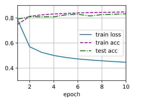
def train_ch3(net,train_iter,test_iter,loss,num_epochs,updater):
    animator = Animator(xlabel='epoch',xlim=[1,num_epochs],ylim=[0.3,0.9],       
                       legend=['train loss','train acc','test acc'])
    for epoch in range(num_epochs):  # 变量num_epochs遍数据
        train_metrics = train_epoch_ch3(net,train_iter,loss,updater) # 返回两个值，一个总损失、一个总正确率
        test_acc = evaluate_accuracy(net, test_iter) # 测试数据集上评估精度，仅返回一个值，总正确率  
        animator.add(epoch+1,train_metrics+(test_acc,)) # train_metrics+(test_acc,) 仅将两个值的正确率相加，
    train_loss, train_acc = train_metrics
    
# 小批量随即梯度下降来优化模型的损失函数
lr = 0.1
def updater(batch_size):
    return d2l.sgd([w,b],lr,batch_size)

#训练模型10个迭代周期
num_epochs = 10
train_ch3(net,train_iter,test_iter,cross_entropy,num_epochs,updater)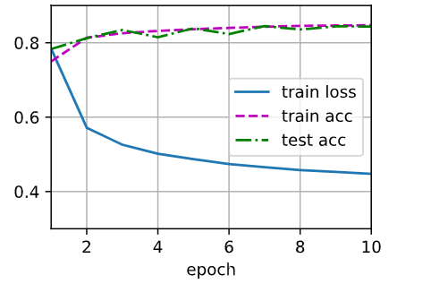

2.10 预测数据

def predict_ch3(net,test_iter,n=6):
    for X, y in test_iter: 
        break # 仅拿出一批六个数据
    trues = d2l.get_fashion_mnist_labels(y)
    preds = d2l.get_fashion_mnist_labels(net(X).argmax(axis=1))
    titles = [true + '\n' + pred for true, pred in zip(trues,preds)]
    d2l.show_images(X[0:n].reshape((n,28,28)),1,n,titles=titles[0:n])
    
predict_ch3(net,test_iter)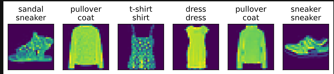

3. Sofmax回归（使用框架）

① 通过深度学习框架的高级API能够使实现softmax回归变得更加容易。

import torch
from torch import nn
from d2l import torch as d2l

batch_size = 256
train_iter, test_iter = d2l.load_data_fashion_mnist(batch_size)

# Softmax回归的输出是一个全连接层
# PyTorch不会隐式地调整输入的形状
# 因此，我们定义了展平层(flatten)在线性层前调整网络输入的形状
net = nn.Sequential(nn.Flatten(),nn.Linear(784,10))

def init_weights(m):
    if type(m) == nn.Linear:
        nn.init.normal_(m.weight, std=0.01) # 方差为0.01

net.apply(init_weights)
print(net.apply(init_weights)) # net网络的参数用的是init_weights初始化参数

# 在交叉熵损失函数中传递未归一化的预测，并同时计算softmax及其对数
loss = nn.CrossEntropyLoss()
# 使用学习率为0.1的小批量随即梯度下降作为优化算法
trainer = torch.optim.SGD(net.parameters(),lr=0.1)

#训练的论数
num_epochs = 10
d2l.train_ch3(net,train_iter,test_iter,loss,num_epochs,trainer)