- 🍨 本文为 🔗365天深度学习训练营中的学习记录博客
- 🍖 原作者: K同学啊
本次任务
- 了解 LSTM 是什么,使用 TensorFlow2 构建一个完整的时序预测程序。
- 数据集提供了火灾温度
Tem1、一氧化碳浓度CO 1、烟雾浓度Soot 1随时间变化的数据,根据这些数据预测未来某一时刻的火灾温度。
- 目标:
R2 >= 0.83。
若未安装 TensorFlow:pip install tensorflow
一、前期准备
1. 导入库与全局配置
import os
import random
import warnings
from datetime import datetime

import matplotlib.pyplot as plt
import numpy as np
import pandas as pd
import tensorflow as tf
from sklearn import metrics
from sklearn.preprocessing import MinMaxScaler

warnings.filterwarnings("ignore")
plt.rcParams["font.sans-serif"] = ["PingFang SC", "Arial Unicode MS", "SimHei", "DejaVu Sans"]
plt.rcParams["axes.unicode_minus"] = False
plt.rcParams["figure.dpi"] = 150

SEED = 123
QUICK_RUN = os.environ.get("QUICK_RUN", "0") == "1"   # QUICK_RUN=1 时快速跑通
EPOCHS = 5 if QUICK_RUN else 20
WINDOW_SIZE = 8


def set_seed(seed=SEED):
    random.seed(seed)
    np.random.seed(seed)
    tf.random.set_seed(seed)


set_seed()
print("TensorFlow:", tf.__version__)

TensorFlow: 2.21.0
2. 导入数据
若当前目录下没有该文件,会自动生成一份模拟火灾数据 以保证流程可完整跑通;放上真实数据后无需改动代码。
def _synthetic_fire(n=6000, seed=SEED):
    """生成模拟火灾时序数据:多次火灾事件(高斯峰)叠加 + 缓慢漂移 + 测量噪声。"""
    rng = np.random.RandomState(seed)
    t = np.arange(n)
    Tem1 = np.full(n, 25.0)  # 室温基线
    for _ in range(25):       # 25 次火灾事件
        c = rng.randint(200, n - 200)
        w = rng.randint(30, 80)
        h = rng.uniform(150, 550)
        Tem1 += h * np.exp(-((t - c) ** 2) / (2 * w ** 2))
    Tem1 += 8 * np.sin(t / 350.0)          # 缓慢漂移
    Tem1 += rng.normal(0, 35, n)           # 测量噪声
    Tem1 = np.clip(Tem1, 20, None)         # 不低于室温
    CO_1 = np.clip(5 + 0.45 * Tem1 + rng.normal(0, 15, n), 0, None)
    Soot_1 = np.clip(2 + 0.30 * Tem1 + rng.normal(0, 12, n), 0, None)
    return pd.DataFrame({"Unnamed: 0": t, "Tem1": Tem1, "CO 1": CO_1, "Soot 1": Soot_1})


def load_fire_data(path="./data/R4-data/woodpine2.csv"):
    if os.path.exists(path):
        df = pd.read_csv(path)
        print(f"[OK] 已加载真实数据:{path}(共 {len(df)} 行)")
    else:
        df = _synthetic_fire()
        print(f"[!] 未找到 {path},已生成模拟火灾数据(共 {len(df)} 行)用于跑通流程。")
    return df


df = load_fire_data()

# 检查各特征列是否含有有效数据(本数据集 CO 1 / Soot 1 可能为 0)
for c in ["Tem1", "CO 1", "Soot 1"]:
    nonzero = (df[c].fillna(0) != 0).mean()
    tag = "有效" if nonzero > 0.01 else "全为 0(无信息量)"
    print(f"  {c:8s}  非零占比 {nonzero*100:5.1f}%   {tag}")

df.head()

[OK] 已加载真实数据:./data/R4-data/woodpine2.csv(共 5948 行)
  Tem1      非零占比 100.0%   有效
  CO 1      非零占比  99.9%   有效
  Soot 1    非零占比  99.9%   有效
|---|-------|------|------|--------|
| | Time | Tem1 | CO 1 | Soot 1 |
| 0 | 0.000 | 25.0 | 0.0 | 0.0 |
| 1 | 0.228 | 25.0 | 0.0 | 0.0 |
| 2 | 0.456 | 25.0 | 0.0 | 0.0 |
| 3 | 0.685 | 25.0 | 0.0 | 0.0 |
| 4 | 0.913 | 25.0 | 0.0 | 0.0 |
3. 数据可视化
注:CO 1 / Soot 1 的原始量纲很小(约 1e-4 量级),与 Tem1 高度相关(相关系数约 0.997)。归一化后量纲差异会被消除,三者对模型都是有效输入。
cols = ["Tem1", "CO 1", "Soot 1"]
units = ["degC", "ppm", "mg/m3"]

fig, axes = plt.subplots(len(cols), 1, figsize=(12, 6), sharex=True)
for ax, col, unit in zip(axes, cols, units):
    ax.plot(df[col], color="steelblue", linewidth=0.8)
    ax.set_ylabel(f"{col} ({unit})")
    ax.grid(alpha=0.3)
axes[-1].set_xlabel("Time step")
fig.suptitle("Fire Temperature / CO / Soot time series", y=1.02)
plt.tight_layout()
plt.show()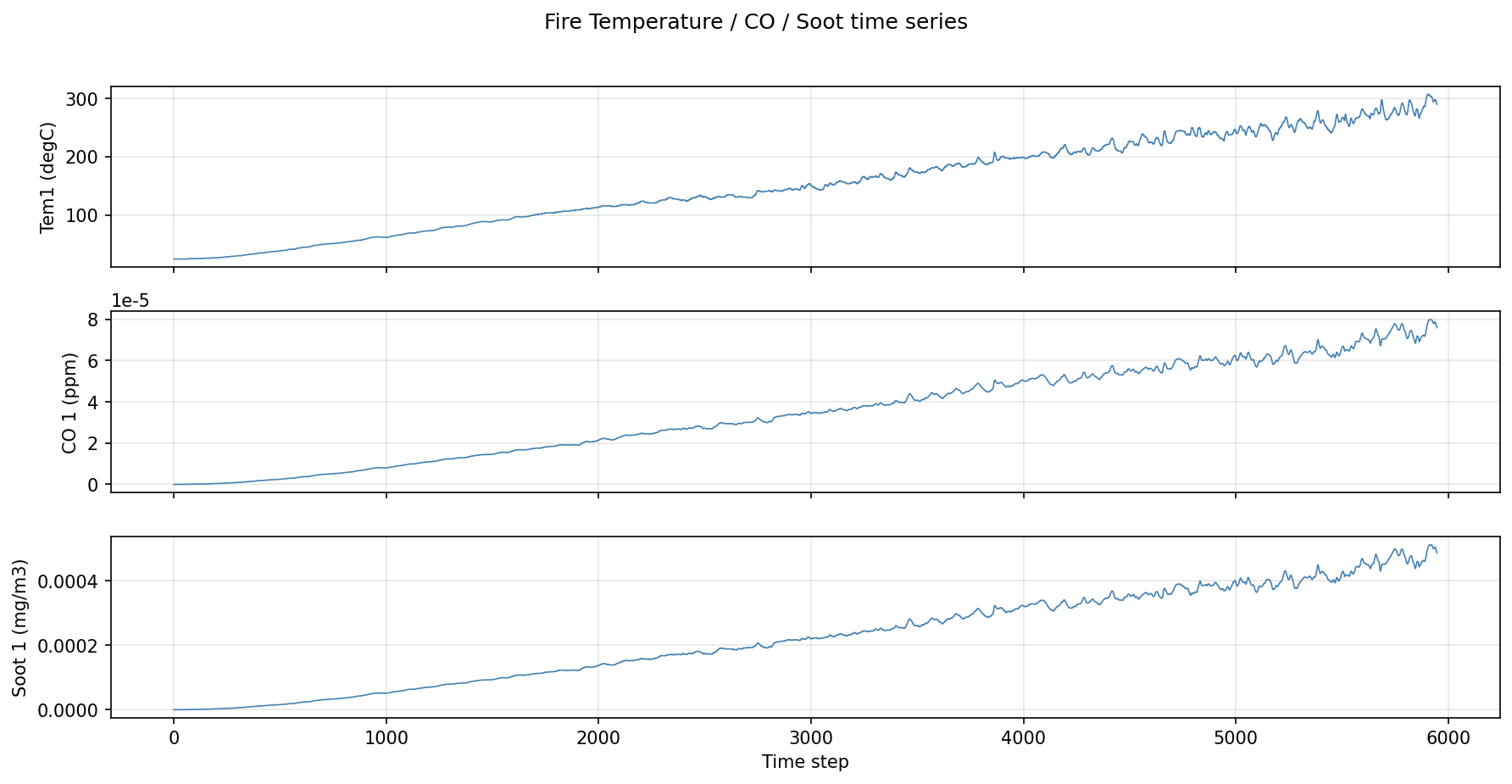
二、构建数据集
1. 设置 X、y(滑动窗口)
取前 8 个时间步的 Tem1、CO 1、Soot 1 作为 X ,第 9 个时间步的 Tem1 作为 y。
data = df[cols].values  # (n, 3)

X, y = [], []
for i in range(len(data) - WINDOW_SIZE):
    X.append(data[i : i + WINDOW_SIZE, :])   # (8, 3)
    y.append(data[i + WINDOW_SIZE, 0])        # 第 9 步的 Tem1

X = np.array(X)
y = np.array(y)
print("X.shape =", X.shape, "(样本数, 时间步, 特征数)")
print("y.shape =", y.shape)

X.shape = (5940, 8, 3) (样本数, 时间步, 特征数)
y.shape = (5940,)
2. 归一化
LSTM 对量纲敏感,使用 MinMaxScaler 将数据缩放到 0, 1。X 按特征维归一化,y 单独归一化(便于预测后还原真实温度)。
scaler_X = MinMaxScaler()
X_scaled = scaler_X.fit_transform(X.reshape(-1, X.shape[-1])).reshape(X.shape)

scaler_y = MinMaxScaler()
y_scaled = scaler_y.fit_transform(y.reshape(-1, 1))

print("X 范围:", round(X_scaled.min(), 3), "~", round(X_scaled.max(), 3))
print("y 范围:", round(y_scaled.min(), 3), "~", round(y_scaled.max(), 3))

X 范围: 0.0 ~ 1.0
y 范围: 0.0 ~ 1.0
3. 划分数据集
时序数据不能随机打乱,按时间顺序划分:第 5000 个样本之前为训练集,之后为验证集。
SPLIT = 5000
X_train, y_train = X_scaled[:SPLIT], y_scaled[:SPLIT]
X_test, y_test = X_scaled[SPLIT:], y_scaled[SPLIT:]

print(f"训练集:X_train {X_train.shape}, y_train {y_train.shape}")
print(f"验证集:X_test  {X_test.shape}, y_test  {y_test.shape}")

训练集:X_train (5000, 8, 3), y_train (5000, 1)
验证集:X_test  (940, 8, 3), y_test  (940, 1)
三、构建模型
LSTM(80):提取 8 个时间步的时序特征。
Dropout(0.2):缓解过拟合。
-
Dense(1):输出下一个时刻的温度(回归任务)。model_lstm = tf.keras.Sequential([
tf.keras.layers.Input(shape=(WINDOW_SIZE, X.shape[-1])),
tf.keras.layers.LSTM(80, activation="tanh"),
tf.keras.layers.Dropout(0.2),
tf.keras.layers.Dense(1),
])model_lstm.summary()
I0000 00:00:1784820479.137412 1503 gpu_device.cc:2043] Created device /job:localhost/replica:0/task:0/device:GPU:0 with 10116 MB memory: -> device: 0, name: NVIDIA GeForce RTX 3080 Ti, pci bus id: 0000:5e:00.0, compute capability: 8.6
Model: "sequential"
┏━━━━━━━━━━━━━━━━━━━━━━━━━━━━━━━━━┳━━━━━━━━━━━━━━━━━━━━━━━━┳━━━━━━━━━━━━━━━┓
┃ Layer (type) ┃ Output Shape ┃ Param # ┃
┡━━━━━━━━━━━━━━━━━━━━━━━━━━━━━━━━━╇━━━━━━━━━━━━━━━━━━━━━━━━╇━━━━━━━━━━━━━━━┩
│ lstm (LSTM) │ (None, 80) │ 26,880 │
├─────────────────────────────────┼────────────────────────┼───────────────┤
│ dropout (Dropout) │ (None, 80) │ 0 │
├─────────────────────────────────┼────────────────────────┼───────────────┤
│ dense (Dense) │ (None, 1) │ 81 │
└─────────────────────────────────┴────────────────────────┴───────────────┘
Total params: 26,961 (105.32 KB)
Trainable params: 26,961 (105.32 KB)
Non-trainable params: 0 (0.00 B)
四、模型训练
1. 编译
回归任务使用均方误差 MSE 作为损失函数,优化器 Adam。
model_lstm.compile(
    optimizer=tf.keras.optimizers.Adam(learning_rate=0.001),
    loss="mean_squared_error",
)
2. 训练
history_lstm = model_lstm.fit(
    X_train, y_train,
    validation_data=(X_test, y_test),
    epochs=EPOCHS,
    batch_size=64,
    verbose=2,
)

Epoch 1/20
I0000 00:00:1784820491.667709    1667 cuda_dnn.cc:461] Loaded cuDNN version 91002
79/79 - 5s - 58ms/step - loss: 0.0120 - val_loss: 8.5372e-04
...
Epoch 20/20
79/79 - 1s - 8ms/step - loss: 5.2048e-04 - val_loss: 2.0036e-04
五、模型评估
1. Loss 曲线
plt.figure(figsize=(6, 3), dpi=120)
plt.plot(history_lstm.history["loss"], label="LSTM Training Loss")
plt.plot(history_lstm.history["val_loss"], label="LSTM Validation Loss")
plt.title(f"Training and Validation Loss  |  {datetime.now():%Y-%m-%d %H:%M}")
plt.xlabel("Epoch")
plt.ylabel("Loss")
plt.legend()
plt.grid(alpha=0.3)
plt.show()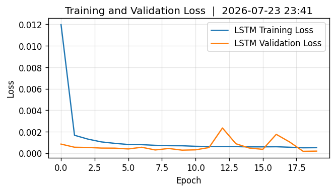
2. 预测值 vs 真实值
预测后需要反归一化还原成真实温度再画图。
predicted_y_lstm = model_lstm.predict(X_test)                       # 归一化空间下的预测
predicted_y_lstm = scaler_y.inverse_transform(predicted_y_lstm)   # 还原为真实温度
y_test_real = scaler_y.inverse_transform(y_test)                  # 真实温度

plt.figure(figsize=(7, 3), dpi=120)
N = 1000
plt.plot(y_test_real[:N], color="red", label="Actual", linewidth=1)
plt.plot(predicted_y_lstm[:N], color="blue", label="Predicted", linewidth=1)
plt.title("Fire Temperature: Actual vs Predicted")
plt.xlabel("Time step")
plt.ylabel("Tem1 (degC)")
plt.legend()
plt.grid(alpha=0.3)
plt.show()

[1m30/30[0m [32m━━━━━━━━━━━━━━━━━━━━[0m[37m[0m [1m0s[0m 5ms/step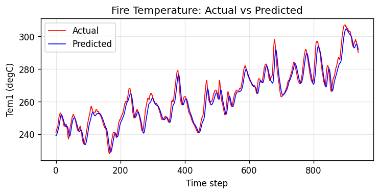
3. 计算 RMSE 与 R2
- RMSE:均方根误差,越小越好。
-
R2:决定系数,越接近 1 越好,目标 >= 0.83。
RMSE_lstm = metrics.mean_squared_error(y_test_real, predicted_y_lstm) ** 0.5
R2_lstm = metrics.r2_score(y_test_real, predicted_y_lstm)print("均方根误差 RMSE: %.5f" % RMSE_lstm)
print("决定系数 R2 : %.5f" % R2_lstm)打卡时间戳
print("evaluated @", datetime.now().strftime("%Y-%m-%d %H:%M:%S"))
均方根误差 RMSE: 3.99167
决定系数 R2 : 0.94399
evaluated @ 2026-07-23 23:29:22
六、多输出时间步(预测第 9~10 时刻)
用前 8 个时刻预测未来 2 个时刻 的 Tem1,只需把 y 改成 2 维、模型输出层改为 Dense(2)。
HORIZON = 2  # 预测未来 2 个时间步

X_m, y_m = [], []
for i in range(len(data) - WINDOW_SIZE - HORIZON + 1):
    X_m.append(data[i : i + WINDOW_SIZE, :])
    y_m.append(data[i + WINDOW_SIZE : i + WINDOW_SIZE + HORIZON, 0])  # 第 9、10 步 Tem1

X_m = np.array(X_m)
y_m = np.array(y_m)

# 复用前面的归一化器
X_m_scaled = scaler_X.transform(X_m.reshape(-1, X_m.shape[-1])).reshape(X_m.shape)
# y_m 形状为 (n, HORIZON),而 scaler_y 是按单列 Tem1 拟合的(仅 1 个特征);
# 两列都是 Tem1,故先展平成 (n*HORIZON, 1) 再归一化,最后还原为 (n, HORIZON)
y_m_scaled = scaler_y.transform(y_m.reshape(-1, 1)).reshape(y_m.shape)

X_m_train, y_m_train = X_m_scaled[:SPLIT], y_m_scaled[:SPLIT]
X_m_test, y_m_test = X_m_scaled[SPLIT:], y_m_scaled[SPLIT:]
print("多步预测 y_train:", y_m_train.shape, "(样本, 预测步数)")

多步预测 y_train: (5000, 2) (样本, 预测步数)

model_multi = tf.keras.Sequential([
    tf.keras.layers.Input(shape=(WINDOW_SIZE, X.shape[-1])),
    tf.keras.layers.LSTM(80, activation="tanh"),
    tf.keras.layers.Dropout(0.2),
    tf.keras.layers.Dense(HORIZON),
])
model_multi.compile(optimizer="adam", loss="mean_squared_error")
model_multi.summary()

history_multi = model_multi.fit(
    X_m_train, y_m_train,
    validation_data=(X_m_test, y_m_test),
    epochs=EPOCHS,
    batch_size=64,
    verbose=2,
)

# 反归一化:预测输出与 y 都是 (n, HORIZON),同样先展平再还原
pred_m = scaler_y.inverse_transform(model_multi.predict(X_m_test).reshape(-1, 1)).reshape(-1, HORIZON)
true_m = scaler_y.inverse_transform(y_m_test.reshape(-1, 1)).reshape(-1, HORIZON)

R2_multi = metrics.r2_score(true_m, pred_m)
print("多步预测 R2: %.5f" % R2_multi)

Model: "sequential_1"
┏━━━━━━━━━━━━━━━━━━━━━━━━━━━━━━━━━┳━━━━━━━━━━━━━━━━━━━━━━━━┳━━━━━━━━━━━━━━━┓
┃ Layer (type)                    ┃ Output Shape           ┃       Param # ┃
┡━━━━━━━━━━━━━━━━━━━━━━━━━━━━━━━━━╇━━━━━━━━━━━━━━━━━━━━━━━━╇━━━━━━━━━━━━━━━┩
│ lstm_1 (LSTM)                   │ (None, 80)             │        26,880 │
├─────────────────────────────────┼────────────────────────┼───────────────┤
│ dropout_1 (Dropout)             │ (None, 80)             │             0 │
├─────────────────────────────────┼────────────────────────┼───────────────┤
│ dense_1 (Dense)                 │ (None, 2)              │           162 │
└─────────────────────────────────┴────────────────────────┴───────────────┘
Total params: 27,042 (105.63 KB)
Trainable params: 27,042 (105.63 KB)
Non-trainable params: 0 (0.00 B)

Epoch 1/20
79/79 - 2s - 20ms/step - loss: 0.0144 - val_loss: 6.8791e-04
...
Epoch 19/20
79/79 - 1s - 8ms/step - loss: 7.0850e-04 - val_loss: 4.1083e-04
Epoch 20/20
79/79 - 1s - 8ms/step - loss: 6.7256e-04 - val_loss: 9.1032e-04
[1m30/30[0m [32m━━━━━━━━━━━━━━━━━━━━[0m[37m[0m [1m0s[0m 5ms/step
多步预测 R2: 0.74521
七、总结
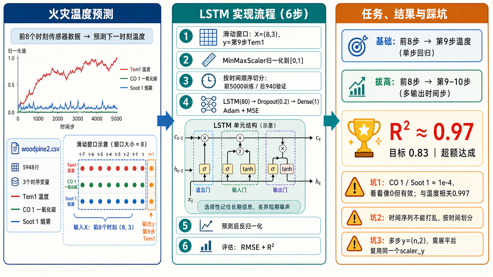
- 完成基于 TensorFlow2 的 LSTM 火灾温度预测:
Tem1 / CO 1 / Soot 1前 8 步 -> 第 9 步温度。
- 关键点:滑动窗口 构造时序样本 ->
MinMaxScaler归一化 -> 按时间顺序划分训练/验证集 -> 预测后反归一化还原。
- 拔高部分把任务升级为多输出时间步(预测第 9~10 步)。