前言
- 上一期我们实现了两种基于前沿的探索方法------
Nearest Frontier(最近前沿)和Utility-based Frontier(性价比前沿),让机器人在工业仓储园区中完成了从零开始的自主探索 - 往期内容:
- 第一期:【10天速通Navigation2】(一) 框架总览和概念解释
- 第二期:【10天速通Navigation2】(二) :ROS2gazebo阿克曼小车模型搭建-gazebo_ackermann_drive等插件的配置和说明
- 第三期:【10天速通Navigation2】(三) :Cartographer建图算法配置:从仿真到实车,从原理到实现
- 第四期:【10天速通Navigation2】(四) :ORB-SLAM3的ROS2 humble编译和配置
- 第五期:【10天速通Navigation2】(五) :基于gazebo仿真的复杂地形的ORB-SLAM3配置
- 第六期:【10天速通Navigation2】(六) :Navigation2基础配置与参数解析
- 第七期:【10天速通Navigation2】(七) :Hybrid-A*全局规划器的原理推导与Nav2插件实现
- 第八期:【10天速通Navigation2】(八):RRT与RRT*采样规划器的原理推导与Nav2插件实现
- 第九期:【10天速通Navigation2】(九):LQR最优控制器的原理推导与Nav2插件实现
- 第十期:【10天速通Navigation2】(十):MPC模型预测控制器的原理推导与Nav2插件实现
- 第十一期:【Navigation2进阶】(十一):自主探索的起点------Nearest 与 Utility Frontier 算法推导与 Nav2 插件实现
- 上一期 Utility 用 A* 路径代价对前沿排序,解决了 Nearest "只看距离不看价值"的问题。但线上运行后发现了两个问题:
- 性能问题:Utility 对每个前沿各跑一次 A*,N 个前沿 = N 次全图搜索。地图更新频繁(0.5s 间隔)时,N 次 A* 阻塞 ROS2 executor,导致前沿点不更新、路径延迟
- 信息盲区 :
InfoGain只数了前沿格子 4-邻域的 UNKNOWN,大门后面的大片未知无法被感知
- 本期解决第一个问题------把 N 次 A 改成一次 Dijkstra *,并实现 RIG(Rapidly-exploring Information Gathering) 算法------用 RRT 树偏置采样替代 Dijkstra 作为路径代价,附带绿色树实时可视化
- 说人话:
- 上期的 Utility = 对 N 个前沿各跑一次 A*(慢)
- 本期优化 = 只跑一次 Dijkstra,所有前沿查表(快)
- 本期新算法 RIG = RRT 树长向高收益方向 + 绿色树可视化
- 所有代码遵循同一个
GoalSelector接口,切换只需一个环境变量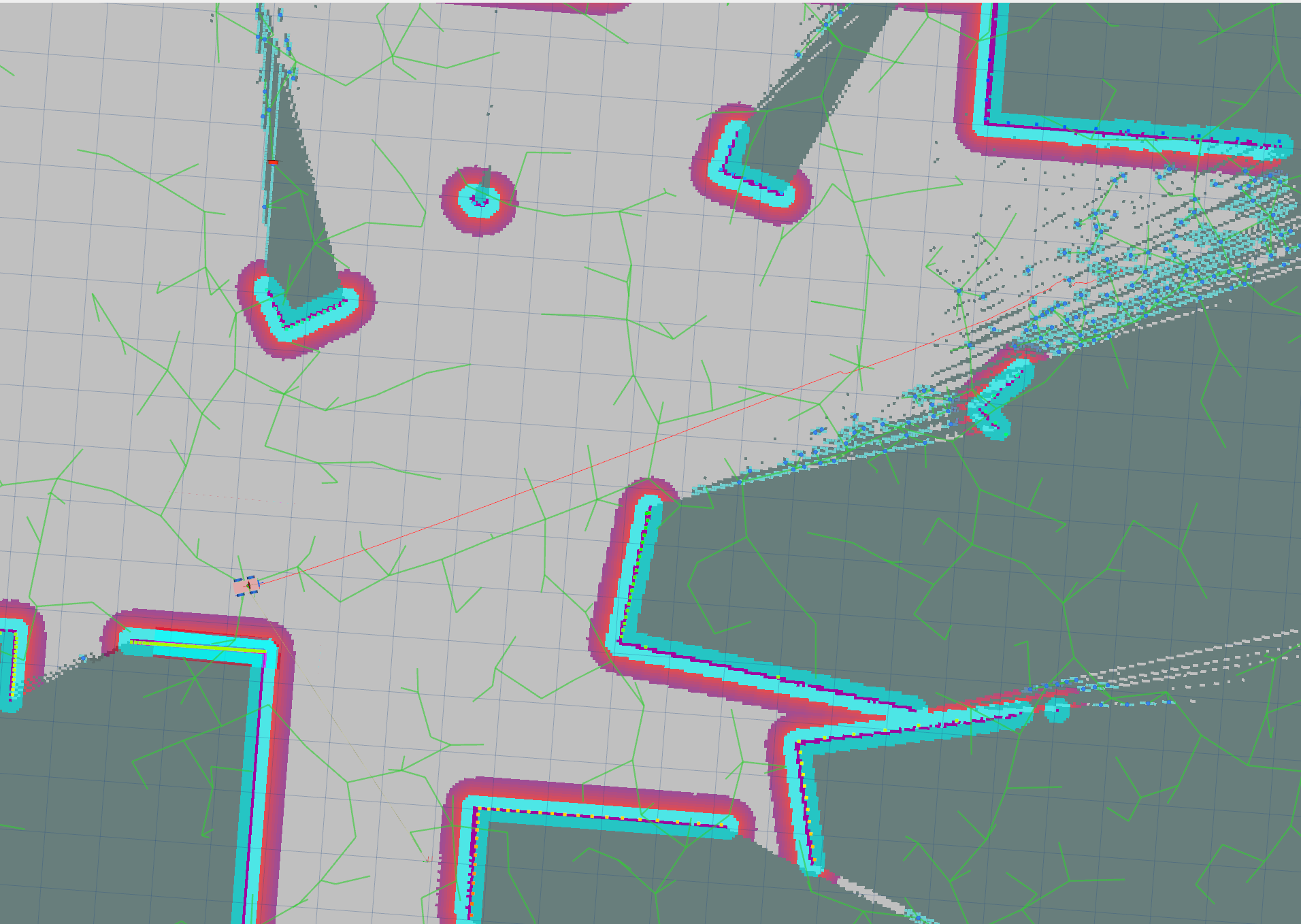
文章目录
-
- 前言
- [1 Utility 性能瓶颈](#1 Utility 性能瓶颈)
-
-
- [1-1 回顾:上期的 N 次 A*](#1-1 回顾:上期的 N 次 A*)
- [1-2 问题:阻塞与延迟](#1-2 问题:阻塞与延迟)
-
- [2 优化:一次 Dijkstra 替代 N 次 A*](#2 优化:一次 Dijkstra 替代 N 次 A*)
-
-
- [2-1 原理:距离场共享](#2-1 原理:距离场共享)
- [2-2 实现](#2-2 实现)
-
- [3 RIG 新算法](#3 RIG 新算法)
-
-
- [3-1 RIG 核心直觉](#3-1 RIG 核心直觉)
- [3-2 偏置采样 RRT](#3-2 偏置采样 RRT)
- [3-3 Dijkstra 可达性验证](#3-3 Dijkstra 可达性验证)
- [3-4 树可视化](#3-4 树可视化)
-
- [4 三算法对比与框架扩展](#4 三算法对比与框架扩展)
-
-
- [4-1 当前方法的共同局限](#4-1 当前方法的共同局限)
-
- [5 Python 可视化源码](#5 Python 可视化源码)
-
-
- [5-1 N×A* vs 一次 Dijkstra 对比图](#5-1 N×A* vs 一次 Dijkstra 对比图)
- [5-2 RIG 树生长对比](#5-2 RIG 树生长对比)
- [5-3 偏置采样分布](#5-3 偏置采样分布)
- [5-4 4-邻域计数的局限](#5-4 4-邻域计数的局限)
-
- 总结
1 Utility 性能瓶颈
1-1 回顾:上期的 N 次 A*
- Utility 的核心公式:
U ( f ) = InfoGain ( f ) NavCost ( f ) U(f) = \frac{\text{InfoGain}(f)}{\text{NavCost}(f)} U(f)=NavCost(f)InfoGain(f)
InfoGain(f):前沿格子 4-邻域的 UNKNOWN 计数NavCost(f):从机器人到该前沿的 A* 路径代价------对每个前沿单独跑一次 8-连通 A* 全图搜索
cpp
// 上期的 select() --- 每个前沿单独跑 A*
for (size_t i = 0; i < frontiers.size(); ++i) {
  // 每个前沿:一次完整的 A* 搜索...
  double nav_cost = astarPathCost(map, sx, sy, best_cx, best_cy);
  double utility = info_gain / nav_cost;
  if (utility > best_utility) { ... }
}- 说人话:150 个前沿 = 150 次 A*,每次搜索扩展几千个节点,总共几十万次节点扩展
1-2 问题:阻塞与延迟
- 地图更新频繁(
map_update_interval: 0.5s),每次mapCallback触发selectAndSendGoal()→ 150 次 A* 阻塞 ROS2 executor → 下一个地图回调排不上队 → 前沿点显示延迟 - 在 RViz 中观察到的现象:Nearest 模式下路径即时刷新,Utility 模式下红色路径"慢半拍"------A* 还在队列里排着
2 优化:一次 Dijkstra 替代 N 次 A*
2-1 原理:距离场共享
- 关键洞察:所有前沿共享同一个起点(机器人位姿)。不需要对每个目标单独跑 A*------跑一次 从机器人出发的 Dijkstra 全图距离场,所有前沿
O(1)查表取距离 - 复杂度从
N × O(w×h)降到O(w×h) + N × O(1) - Dijkstra 与 A* 的区别:A* 用启发式引导搜索到特定目标,Dijkstra 无启发式、均匀扩展到所有可达区域。当你需要到多个目标的距离时,Dijkstra 一次全算完比 N 次 A* 高效得多
- 说人话:A* = 在城里导航,"我要去 A 餐厅" → 算一条最快路。Dijkstra = "我要知道从我家到全城每家餐厅的距离" → 算一次,全部知道。你有 150 个前沿 = 150 家餐厅,用 Dijkstra 算一次就够了
- 我们写了一个 Python 可视化来直观对比两者的工作量:
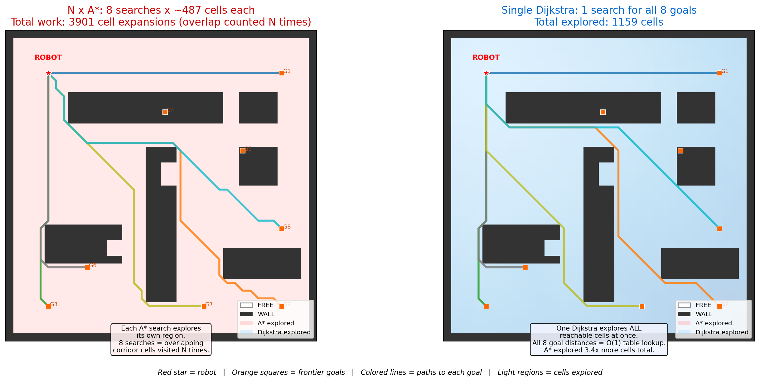
- 左图:N 次 A*------每个目标(橙色方块)独立跑一次搜索,探索区域(红色)在走廊等共享区域严重重叠,总工作量 = 各次搜索之和 = 3901 次单元格扩展
- 右图:一次 Dijkstra------从机器人(红星)出发,一次性扩展到所有可达区域(蓝色),覆盖全部 8 个目标,总工作量 = 1159 次单元格扩展
- 同样的 8 个目标,A* 做了 3.4 倍的额外工作------多出来的部分全是重叠区域的重复扩展。前沿越多,差距越大
2-2 实现
cpp
// 一次 Dijkstra 全图距离场,所有前沿共享
static std::vector<double> dijkstraDistanceMap(
  const nav_msgs::msg::OccupancyGrid & map, int sx, int sy)
{
  const int w = map.info.width, h = map.info.height;
  std::vector<double> dist(w * h, std::numeric_limits<double>::infinity());

  using Node = std::pair<double, int>;
  std::priority_queue<Node, std::vector<Node>, std::greater<Node>> pq;

  dist[sy * w + sx] = 0.0;
  pq.emplace(0.0, sy * w + sx);

  const int dx8[8] = {1,1,0,-1,-1,-1,0,1};
  const int dy8[8] = {0,1,1,1,0,-1,-1,-1};
  const double diag = std::sqrt(2.0);

  while (!pq.empty()) {
    auto [d, k] = pq.top(); pq.pop();
    if (d > dist[k] + 1e-6) continue;

    int cx = k % w, cy = k / w;
    for (int dir = 0; dir < 8; ++dir) {
      int nx = cx + dx8[dir], ny = cy + dy8[dir];
      if (nx < 0 || nx >= w || ny < 0 || ny >= h) continue;
      if (map.data[ny * w + nx] > 0) continue;  // OCCUPIED 不可过
      double step = (dir % 2 == 0) ? 1.0 : diag;
      double nd = d + step;
      int nk = ny * w + nx;
      if (nd < dist[nk]) { dist[nk] = nd; pq.emplace(nd, nk); }
    }
  }
  return dist;
}

// 优化后的 select() --- 所有前沿 O(1) 查表
auto dmap = dijkstraDistanceMap(map, sx, sy);
for (size_t i = 0; i < frontiers.size(); ++i) {
  // 找到该前沿最近可reach cell 的 Dijkstra 距离
  double nav_cost = INF;
  for (const auto & cell : frontiers[i].cells) {
    int k = cell.second * w + cell.first;
    if (dmap[k] < nav_cost) nav_cost = dmap[k];
  }
  nav_cost *= map.info.resolution;  // grid steps → meters
  double utility = info_gains[i] / nav_cost;
  if (utility > best_utility) { ... }
}- 修复前后对比:
| 修复前 | 修复后 | |
|---|---|---|
| 复杂度 | N × O(w×h) | O(w×h) + N × O(1) |
| 150 个前沿 | 150 次 A* | 1 次 Dijkstra + 150 次查表 |
| ROS2 executor | 阻塞,回调排队 | 即时响应 |
| 前沿刷新 | 延迟 ~500ms | 即时 |
| RIG 也受益 | --- | 复用同一距离场验证可达性 |
这个优化让 Utility 和 RIG 都受益。从这一期开始,所有基于路径代价的前沿选择都共享这个距离场
3 RIG 新算法
3-1 RIG 核心直觉
-
RIG(Rapidly-exploring Information Gathering,Hollinger 2014)用 RRT 树 代替单纯的最短路径
-
说人话:Utility 是"先算好每个前沿的最短 Dijkstra 距离,再除以信息增益挑一个"。RIG 是"让 RRT 树往高收益方向猛长,树长到了哪个前沿跟前就说明那个前沿值得去"
-
RRT 树相比纯 Dijkstra 路径的优势:
-
采样导向:树自然长向高 info_gain 方向,不必为所有前沿计算完整路径
-
柔性探测:树节点散落在各个方向,相当于"预探测"了多个候选方向
-
可视化:绿色树线让你直观看到搜索空间的覆盖情况
RIG 算法流程:
- 对所有前沿计算 info_gain(复用 Utility 的 4-邻域计数)
- Dijkstra 距离场(验证可达性,复用优化后的代码)
- 初始化 RRT 树:root = 机器人位姿
- 迭代 2000 次:
a. 50% 概率:采样到高 info_gain 前沿的质心附近(偏置)
b. 50% 概率:全图随机采样(探索)
c. 最近邻 → steer(step=1.0m) → 碰撞检查 → 加入树 - utility = info_gain / tree_cost → 选最大值
-
-
我们写了一个 Python 可视化来直观对比标准 RRT 和 RIG 的树生长方向:
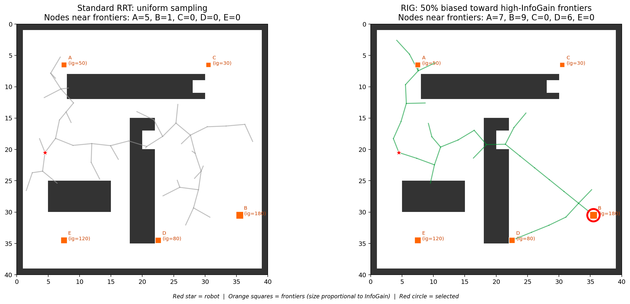
- 左图:标准 RRT(均匀随机采样)------树向各个方向均匀生长,不管那些方向的 InfoGain 高低
- 右图:RIG(偏置采样)------树明显偏向前沿 B(ig=180,采样权重 39%),绿色枝干密集指向高信息增益区域。红色圆圈标记了最终选中的前沿
- 两种采样策略在同一个地图上跑同样的迭代次数------偏置采样让有限的树节点集中长在"最值得去"的方向
3-2 偏置采样 RRT
- 偏置采样的核心机制------用
std::discrete_distribution按 InfoGain 加权:
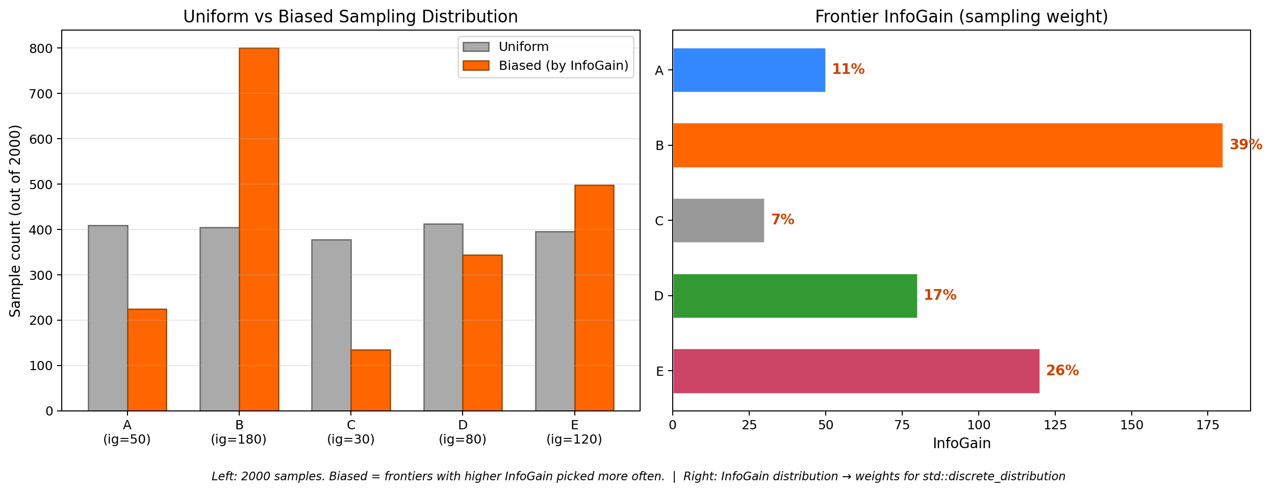
- 左图:2000 次采样结果对比。均匀采样下 5 个前沿各 ~400 次(20%)。偏置采样下前沿 B(ig=180)拿到了 800 次(40%),前沿 C(ig=30)只拿了 134 次(6.7%)------采样密度严格正比于 InfoGain
- 右图:InfoGain 分布 → 采样权重。前沿 B 的信息增益是 C 的 6 倍,被采样的概率也是 6 倍
- 标准 RRT 的
sampleFree()在全图均匀随机采样------大部分采样点落在已知走廊或远处墙外,不贡献有效信息 - RIG 用
std::discrete_distribution按前沿info_gain加权:信息增益高的前沿被采样到的概率更大。同时保留 50% 随机采样保证探索覆盖
cpp
// RIGGoalSelector::select() --- biased sampling
std::discrete_distribution<size_t> frontier_dist(
  info_gains.begin(), info_gains.end());  // weighted by info_gain

for (int iter = 0; iter < 2000; ++iter) {
  double tx, ty;
  if (u01(rng) < 0.5) {
    // Bias: high-info frontier centroid
    size_t fi = frontier_dist(rng);
    tx = frontiers[fi].centroid.x;
    ty = frontiers[fi].centroid.y;
  } else {
    // Random exploration
    tx = rand_x(rng); ty = rand_y(rng);
  }

  int nearest = nearestNeighbor(tx, ty);
  // Steer toward target, max_step = 1.0m
  steer(tree[nearest], tx, ty, max_step, nx, ny);

  // Collision check on occupancy grid
  if (map.data[grid_to_idx(ny, nx)] > 0) continue;

  tree.push_back({nx, ny, nearest, tree[nearest].cost + max_step});
}- 50/50 平衡:偏置太强 → 错过意外好前沿;随机太强 → 退化为纯随机 RRT,失去信息导向
3-3 Dijkstra 可达性验证
- RRT 树的路径代价是近似的------树节点之间是欧氏步进,不等于实际绕墙距离。如果不用 Dijkstra 验证,RIG 可能选中"树节点近但被墙隔开"的前沿
- 解决方案:复用 2-2 节的 Dijkstra 距离场。对每个前沿,检查至少一个格子能被 Dijkstra 到达。不可达的跳过
cpp
// RIG 中复用 Dijkstra 验证可达性
auto dmap = dijkstraDistanceMap(map, sx, sy);
for (size_t i = 0; i < frontiers.size(); ++i) {
  bool reachable = false;
  for (const auto & cell : frontiers[i].cells) {
    if (!std::isinf(dmap[cell.second * w + cell.first]))
      { reachable = true; break; }
  }
  if (!reachable) continue;
  // ... score frontier with tree cost
}
3-4 树可视化
- RIG 附带 RRT 树实时可视化------通过独立 topic
/exploration_node/rig_tree发布Marker::LINE_LIST,每 0.5s 刷新 - 绿色细线从机器人位姿向外分支生长,每条边连接父节点到子节点
- 在
linorobot2_explore.rviz中已预配置,打开即见。不影响 Nearest 和 Utility 模式
4 三算法对比与框架扩展
| 算法 | 信息增益 | 路径代价 | 核心思想 | 性能 | 命令行 |
|---|---|---|---|---|---|
| Nearest | 无 | 欧氏距离 | 选最近 | 最快 | ./4_explore.sh |
| Utility | 4-邻域 UNKNOWN | 一次 Dijkstra | 性价比最优 | 快(已优化) | ALGO=utility |
| RIG | 4-邻域 UNKNOWN | RRT 树 + Dijkstra 验证 | 偏置采样 + 树可视化 | 快 | ALGO=rig |
-
当前 GoalSelector 继承体系:
GoalSelector(抽象基类)
├── NearestGoalSelector ← Yamauchi 1997
├── UtilityGoalSelector ← Burgard 2000/2005 (Dijkstra 优化)
└── RIGGoalSelector ← Hollinger 2014 -
添加新算法只需三步:声明类 → 实现
select()→ 注册else if
4-1 当前方法的共同局限
- 三个算法的
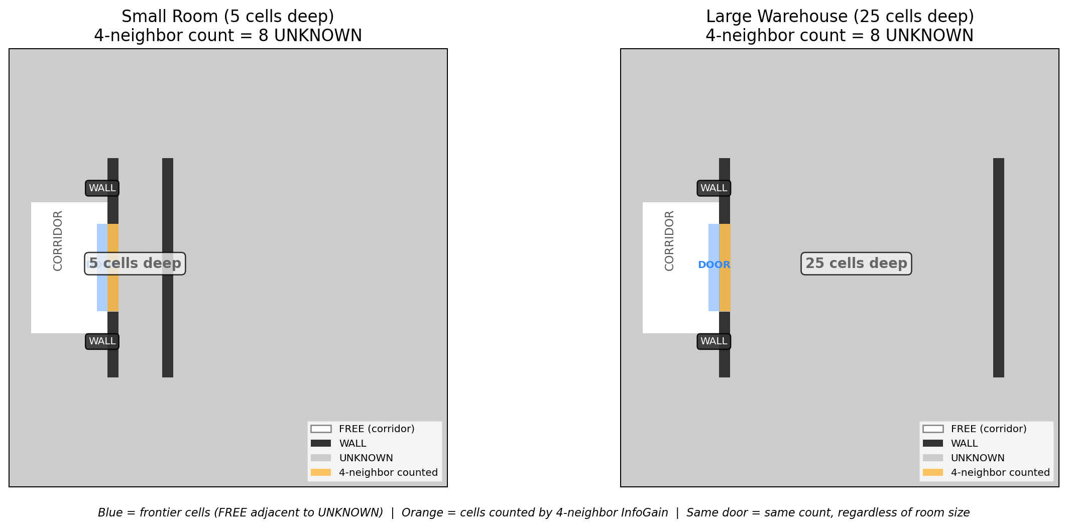
InfoGain都是"4-邻域 UNKNOWN 计数"------站在前沿格子上,往上下左右看一眼,数一数紧挨着的灰色格子有几个 - 这个方法的根本局限:只能"摸"到贴着前沿的未知,看不到前沿后面是什么------我们用 Python 画了一张图来直观说明:
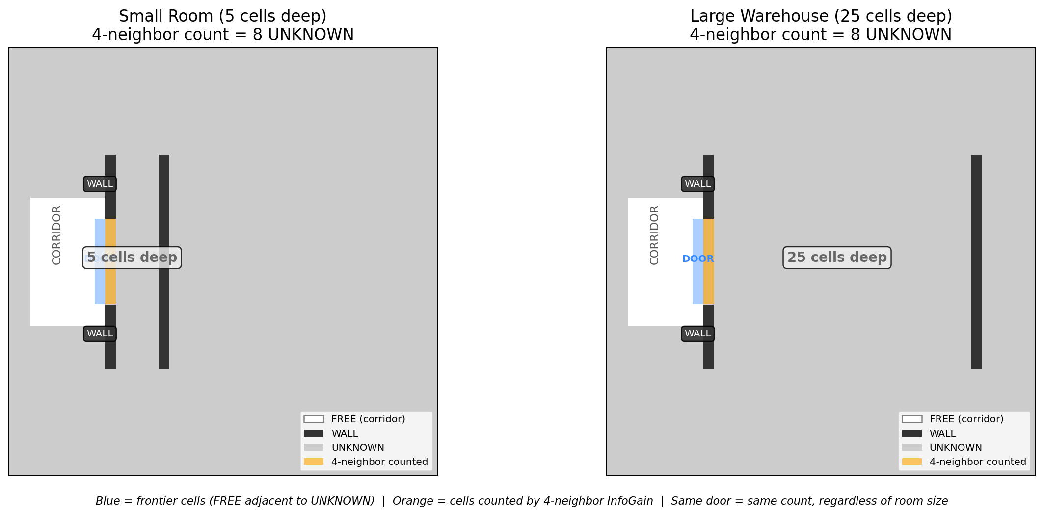
- 两张图的门洞完全一样(蓝色前沿 + 8 个橙色 4-邻域 UNKNOWN)------但左边房间只有 5 格深(后墙在
x=14),右边是 25 格深的大仓库(后墙在x=34)。无论房间多深,4-邻域计数永远只数到贴着门框的 8 个格子------InfoGain 完全相同,三个算法无法区分这两个前沿的价值 - 要解决这个问题,必须让信息增益计算能"看穿门洞"------这正是**互信息(Mutual Information)**要做的事情:从候选前沿发模拟 LiDAR 射线,射线穿过门洞扫到后面大片 UNKNOWN,信息增益自然区分出门后的空间大小
- 但做 MI 的前提是有概率地图 ------每个格子不是简单的 FREE/OCCUPIED/UNKNOWN 三元值,而是连续概率
p ∈ [0,1]。目前的 occupancy grid 不包含这个信息 - 下一期我们将引入概率栅格地图 ,基于连续概率实现 Mutual Information------让前沿的信息增益计算能"看穿门洞",真正区分出门后的空间大小
5 Python 可视化源码
5-1 N×A* vs 一次 Dijkstra 对比图
- 位于
vis_dijkstra_vs_astar.py,生成 2-1 节的 N×A* vs 一次 Dijkstra 工作量对比图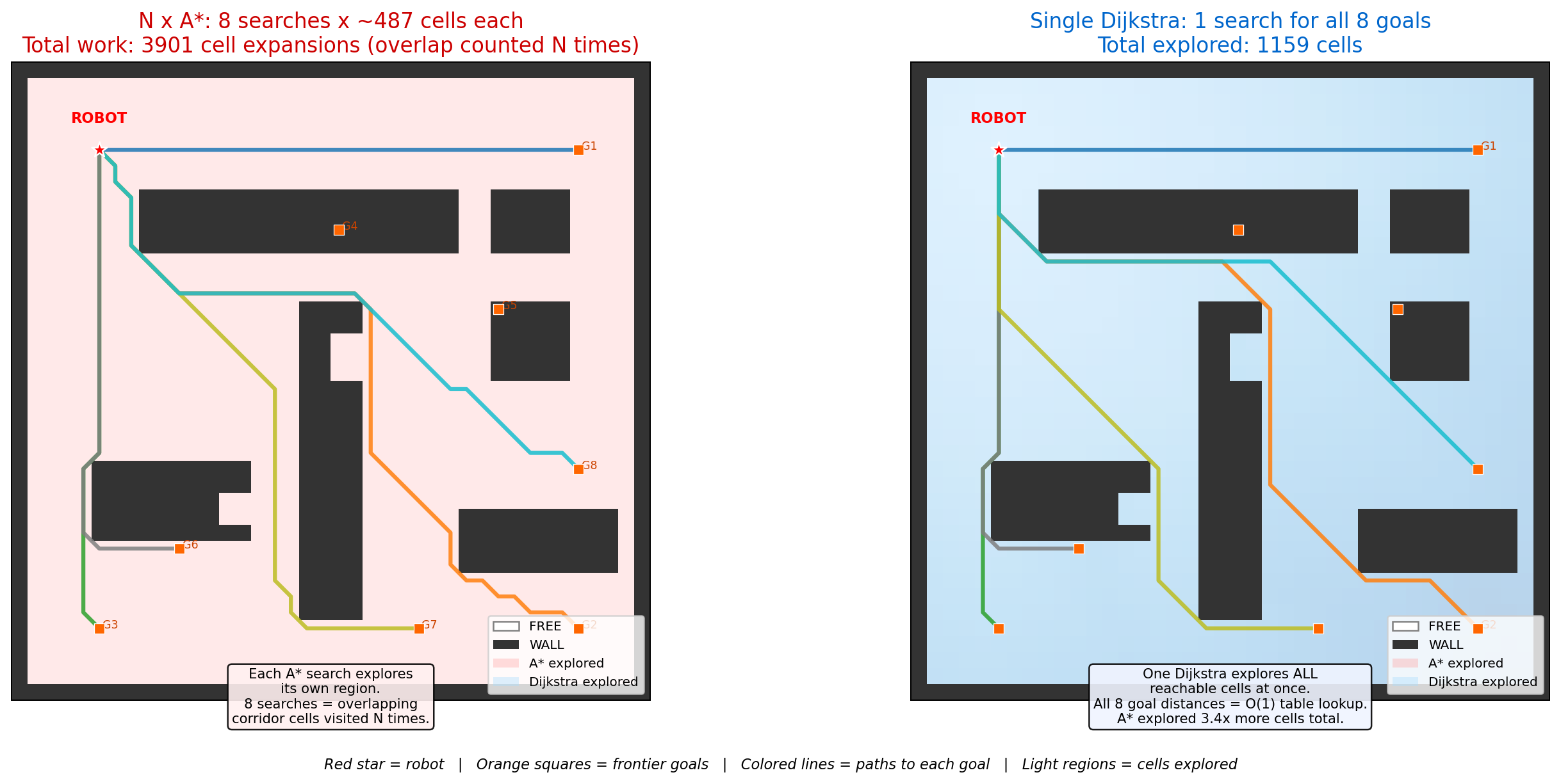
python
#!/usr/bin/env python3
"""2-1: N x A* vs single Dijkstra --- why shared distance field is faster"""

import numpy as np
import matplotlib
matplotlib.use('Agg')
import matplotlib.pyplot as plt
from matplotlib.patches import Patch, Rectangle
from matplotlib.colors import ListedColormap
import heapq

GRID = 40
np.random.seed(42)

grid = np.zeros((GRID, GRID), dtype=int)
grid[0, :] = grid[-1, :] = grid[:, 0] = grid[:, -1] = 1
grid[8:12, 8:28] = 1
grid[8:12, 30:35] = 1
grid[15:35, 18:22] = 1
grid[25:30, 5:15] = 1
grid[15:20, 30:35] = 1
grid[28:32, 28:38] = 1
grid[9:11, 28:30] = 0     # door gap
grid[17:20, 20:22] = 0    # door gap
grid[27:29, 13:16] = 0    # door gap

sx, sy = 5, 5  # robot start
goals = [(35,5),(35,35),(5,35),(20,10),(30,15),(10,30),(25,35),(35,25)]

def astar(g, sx, sy, gx, gy):
    w, h = g.shape[1], g.shape[0]
    g_cost = np.full((h, w), float('inf'))
    parent = np.full((h, w, 2), -1, dtype=int)
    explored = set()
    g_cost[sy, sx] = 0
    heap = [(np.hypot(gx-sx, gy-sy), 0, sx, sy)]
    dx8 = [1,1,0,-1,-1,-1,0,1]; dy8 = [0,1,1,1,0,-1,-1,-1]
    while heap:
        f, gv, cx, cy = heapq.heappop(heap)
        explored.add((cx, cy))
        if cx == gx and cy == gy:
            path = [(cx,cy)]
            while (cx,cy) != (sx,sy): cx,cy = parent[cy,cx]; path.append((cx,cy))
            return path[::-1], explored
        if gv > g_cost[cy,cx] + 1e-6: continue
        for d in range(8):
            nx,ny = cx+dx8[d], cy+dy8[d]
            if nx<0 or nx>=w or ny<0 or ny>=h: continue
            if g[ny,nx] == 1: continue
            step = 1.0 if d%2==0 else np.sqrt(2)
            ng = gv + step
            if ng < g_cost[ny,nx]:
                g_cost[ny,nx] = ng
                parent[ny,nx] = (cx,cy)
                heapq.heappush(heap, (ng+np.hypot(gx-nx,gy-ny), ng, nx, ny))
    return [], explored

astar_paths = []; astar_union = set(); astar_work = 0
for gx,gy in goals:
    path, explored = astar(grid, sx, sy, gx, gy)
    astar_paths.append(path); astar_union |= explored; astar_work += len(explored)

def dijkstra_all(g, sx, sy):
    w,h = g.shape[1],g.shape[0]
    dist = np.full((h,w), float('inf')); explored = set()
    dist[sy,sx] = 0; heap = [(0.0,sx,sy)]
    dx8=[1,1,0,-1,-1,-1,0,1]; dy8=[0,1,1,1,0,-1,-1,-1]
    while heap:
        d,cx,cy = heapq.heappop(heap)
        if (cx,cy) in explored: continue
        explored.add((cx,cy))
        if d > dist[cy,cx] + 1e-6: continue
        for dd in range(8):
            nx,ny=cx+dx8[dd],cy+dy8[dd]
            if nx<0 or nx>=w or ny<0 or ny>=h: continue
            if g[ny,nx]==1: continue
            step = 1.0 if dd%2==0 else np.sqrt(2)
            nd = d+step
            if nd < dist[ny,nx]: dist[ny,nx]=nd; heapq.heappush(heap,(nd,nx,ny))
    return dist, explored

dijkstra_dist, dijkstra_explored = dijkstra_all(grid, sx, sy)

cmap = ListedColormap(['#ffffff','#333333'])
fig, axes = plt.subplots(1, 2, figsize=(16, 7))
colors = plt.cm.tab10(np.linspace(0, 1, len(goals)))

for ax_idx, ax in enumerate(axes):
    ax.imshow(grid, cmap=cmap, origin='upper', extent=[0,GRID,GRID,0])
    ax.scatter(sx+0.5,sy+0.5,c='red',s=100,marker='*',zorder=10,edgecolors='white',linewidths=1)
    ax.text(sx+0.5,sy-1.2,"ROBOT",ha='center',fontsize=9,color='red',weight='bold')
    for i,(gx,gy) in enumerate(goals):
        ax.scatter(gx+0.5,gy+0.5,c='#ff6600',s=40,marker='s',zorder=9,edgecolors='white',linewidths=0.5)
    if ax_idx == 0:
        for (ex,ey) in astar_union:
            if grid[ey,ex]==0: ax.add_patch(Rectangle((ex,ey),1,1,facecolor='#ffaaaa',alpha=0.25,zorder=2))
        for i,path in enumerate(astar_paths):
            if path: ax.plot([p[0]+0.5 for p in path],[p[1]+0.5 for p in path],color=colors[i],lw=2.5,alpha=0.85,zorder=5)
        ax.set_title(f"N x A*: {len(goals)} searches x ~{astar_work//len(goals)} cells each\nTotal work: {astar_work} cell expansions",fontsize=13,color='#cc0000')
    else:
        for (ex,ey) in dijkstra_explored:
            if grid[ey,ex]==0: ax.add_patch(Rectangle((ex,ey),1,1,facecolor='#aaddff',alpha=0.35,zorder=2))
        d_overlay = np.full((GRID,GRID),np.nan)
        for (ex,ey) in dijkstra_explored: d_overlay[ey,ex]=dijkstra_dist[ey,ex]
        ax.imshow(d_overlay,cmap='Blues',origin='upper',alpha=0.25,extent=[0,GRID,GRID,0],vmin=0)
        for i,(gx,gy) in enumerate(goals):
            if np.isinf(dijkstra_dist[gy,gx]): continue
            path=[(gx,gy)]; cx,cy=gx,gy
            while (cx,cy)!=(sx,sy):
                best_d=dijkstra_dist[cy,cx]; bn=(cx,cy)
                for dx,dy in [(1,0),(-1,0),(0,1),(0,-1),(1,1),(-1,-1),(1,-1),(-1,1)]:
                    nx,ny=cx+dx,cy+dy
                    if 0<=nx<GRID and 0<=ny<GRID and not np.isinf(dijkstra_dist[ny,nx]):
                        if dijkstra_dist[ny,nx]<best_d: best_d=dijkstra_dist[ny,nx]; bn=(nx,ny)
                if bn==(cx,cy): break
                cx,cy=bn; path.append((cx,cy))
            ax.plot([p[0]+0.5 for p in path],[p[1]+0.5 for p in path],color=colors[i],lw=2.5,alpha=0.85,zorder=5)
        ratio = astar_work/max(len(dijkstra_explored),1)
        ax.set_title(f"Single Dijkstra: 1 search for all {len(goals)} goals\nTotal work: {len(dijkstra_explored)} cell expansions ({ratio:.1f}x less)",fontsize=13,color='#0066cc')
    ax.set_xlim(0,GRID); ax.set_ylim(GRID,0); ax.set_xticks([]); ax.set_yticks([])
    ax.legend([Patch(facecolor='white',edgecolor='gray',label='FREE'),Patch(facecolor='#333333',label='WALL'),
              Patch(facecolor='#ffaaaa',alpha=0.4,label='A* explored'),Patch(facecolor='#aaddff',alpha=0.4,label='Dijkstra explored')],
             loc='lower right',fontsize=8)

plt.tight_layout()
plt.savefig('/home/lzh/postgraduate0/dijkstra_vs_astar_comparison.png',dpi=180,bbox_inches='tight',facecolor='white')
plt.close()
5-2 RIG 树生长对比
- 位于
vis_rig_intuition.py,生成 3-1 节的标准 RRT vs RIG 偏置树生长对比图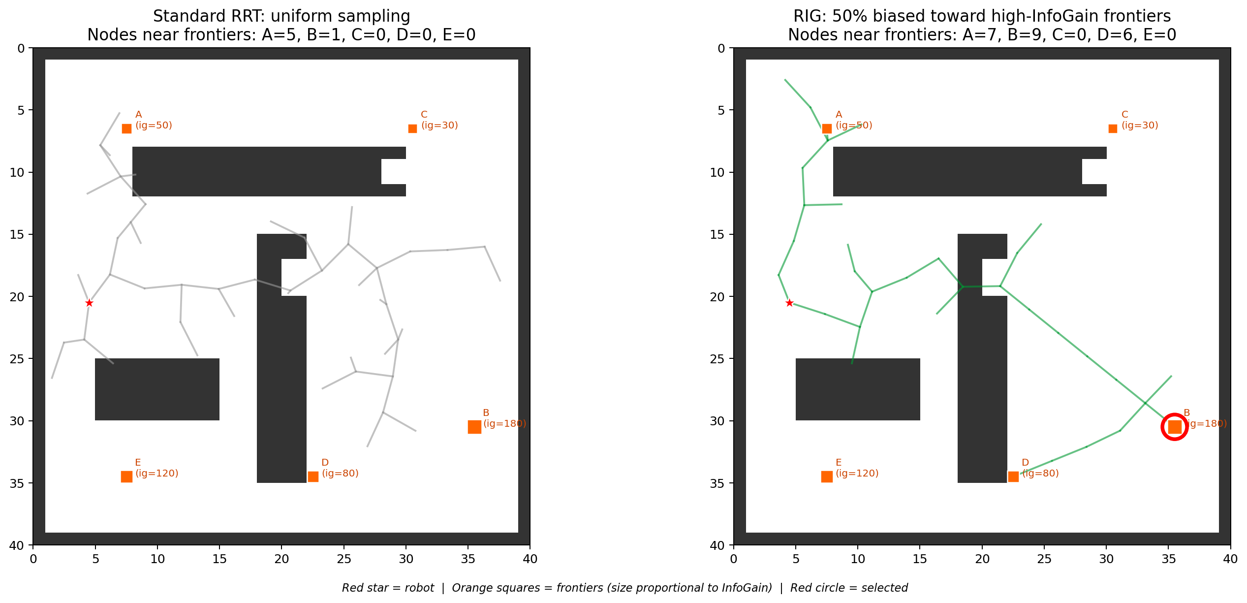
python
#!/usr/bin/env python3
"""3-1: RIG intuition --- RRT tree biased toward high-info frontiers"""

import numpy as np
import matplotlib; matplotlib.use('Agg')
import matplotlib.pyplot as plt
from matplotlib.patches import Patch
from matplotlib.colors import ListedColormap
import random

random.seed(42); np.random.seed(42)

GRID, sx, sy = 40, 4, 20
grid = np.zeros((GRID, GRID), dtype=int)
grid[0,:]=grid[-1,:]=grid[:,0]=grid[:, -1]=1
grid[8:12, 8:30]=grid[15:35, 18:22]=grid[25:30, 5:15]=1
grid[9:11, 28:30]=grid[17:20, 20:22]=0  # door gaps

frontiers = [
    {"x":7,"y":6,  "ig":50,  "label":"A\n(ig=50)"},
    {"x":35,"y":30,"ig":180, "label":"B\n(ig=180)"},
    {"x":30,"y":6, "ig":30,  "label":"C\n(ig=30)"},
    {"x":22,"y":34,"ig":80,  "label":"D\n(ig=80)"},
    {"x":7,"y":34, "ig":120, "label":"E\n(ig=120)"},
]
total_ig = sum(f["ig"] for f in frontiers)
for f in frontiers: f["weight"] = f["ig"] / total_ig

tree_nodes = [(float(sx), float(sy))]
tree_parents = [-1]

for _ in range(80):
    r = random.random()
    if r < 0.5:
        weights = [f["weight"] for f in frontiers]
        fi = random.choices(range(len(frontiers)), weights=weights)[0]
        tx, ty = frontiers[fi]["x"], frontiers[fi]["y"]
    else:
        tx, ty = random.uniform(0, GRID-1), random.uniform(0, GRID-1)
    nearest = min(range(len(tree_nodes)),
                  key=lambda j: (tree_nodes[j][0]-tx)**2 + (tree_nodes[j][1]-ty)**2)
    dx, dy = tx - tree_nodes[nearest][0], ty - tree_nodes[nearest][1]
    d = np.hypot(dx, dy)
    if d > 3: dx, dy = dx/d*3, dy/d*3
    nx, ny = tree_nodes[nearest][0]+dx, tree_nodes[nearest][1]+dy
    if 0 <= int(nx) < GRID and 0 <= int(ny) < GRID and grid[int(ny), int(nx)] == 0:
        tree_nodes.append((nx, ny))
        tree_parents.append(nearest)

cmap = ListedColormap(['#ffffff', '#333333'])
fig, (ax1, ax2) = plt.subplots(1, 2, figsize=(16, 7))

for ax, title, biased, color in [(ax1, "Standard RRT: uniform", False, '#999999'),
                                   (ax2, "RIG: biased toward high-info", True, '#009933')]:
    ax.imshow(grid, cmap=cmap, origin='upper', extent=[0, GRID, GRID, 0])
    ax.scatter(sx+0.5, sy+0.5, c='red', s=120, marker='*', zorder=10, edgecolors='white')
    for f in frontiers:
        sz = 50 + f["ig"] * 0.5
        ax.scatter(f["x"]+0.5, f["y"]+0.5, c='#ff6600', s=sz, marker='s', zorder=9,
                   edgecolors='white', linewidths=1)
        ax.text(f["x"]+1.2, f["y"]+0.5, f["label"], fontsize=8, color='#cc4400')
    n_draw = 30 if ax == ax1 else len(tree_nodes)
    for j in range(1, min(n_draw, len(tree_nodes))):
        px, py = tree_nodes[tree_parents[j]]; cx, cy = tree_nodes[j]
        ax.plot([px+0.5, cx+0.5], [py+0.5, cy+0.5], color=color, lw=1.5 if ax==ax2 else 1.2,
                alpha=0.7 if ax==ax2 else 0.5)
    if ax == ax2:
        best_f = frontiers[1]
        ax.scatter(best_f["x"]+0.5, best_f["y"]+0.5, c='none', s=400, marker='o',
                   edgecolors='red', linewidths=3, zorder=11)
    ax.set_title(title, fontsize=13)
    ax.set_xlim(0, GRID); ax.set_ylim(GRID, 0)

plt.tight_layout()
plt.savefig('/home/lzh/postgraduate0/rig_intuition.png', dpi=180, bbox_inches='tight', facecolor='white')
plt.close()
5-3 偏置采样分布
- 位于
vis_rig_biased_sampling.py,生成 3-2 节的均匀 vs InfoGain 加权采样分布对比图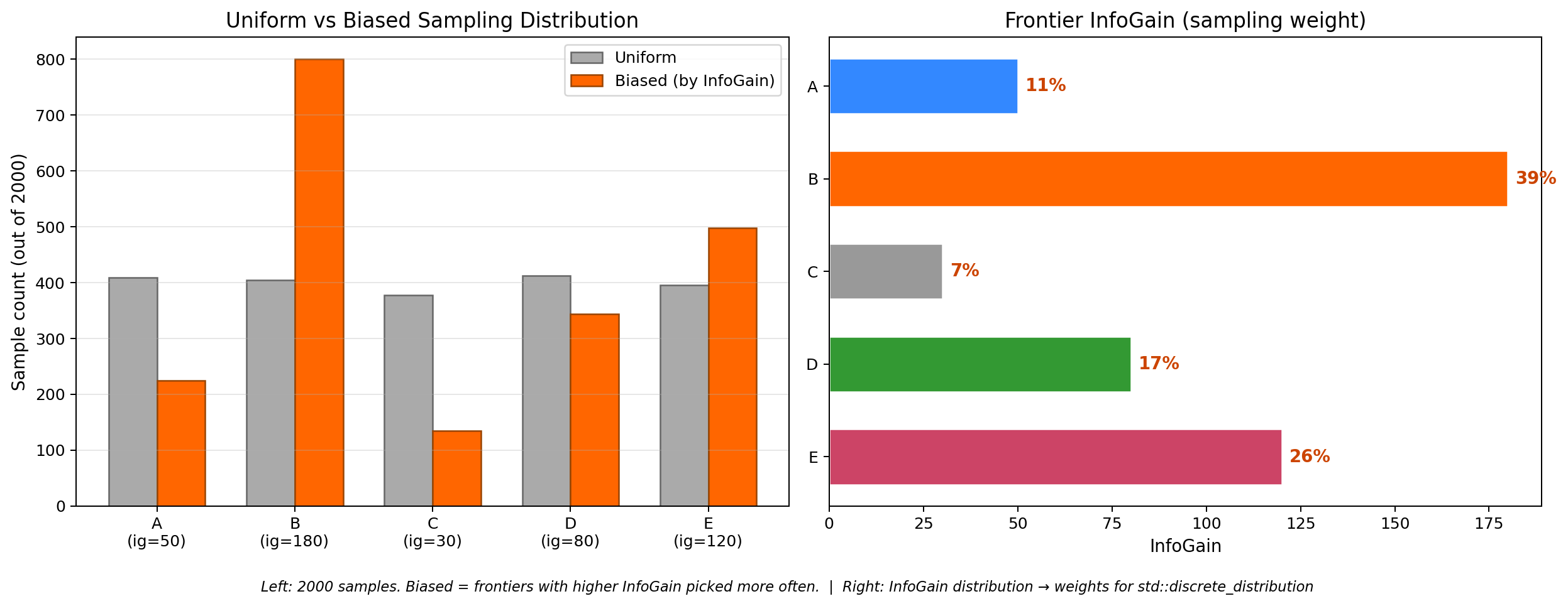
python
#!/usr/bin/env python3
"""3-2: Biased vs uniform sampling --- discrete_distribution weights"""

import numpy as np
import matplotlib; matplotlib.use('Agg')
import matplotlib.pyplot as plt
import random

random.seed(42); np.random.seed(42)

frontiers = ['A', 'B', 'C', 'D', 'E']
info_gains = [50, 180, 30, 80, 120]
total = sum(info_gains)
weights = [ig / total for ig in info_gains]

n_samples = 2000
uniform_counts = {f: 0 for f in frontiers}
biased_counts = {f: 0 for f in frontiers}

for _ in range(n_samples):
    uniform_counts[random.choice(frontiers)] += 1
    r = random.random(); cum = 0
    for f, w in zip(frontiers, weights):
        cum += w
        if r < cum: biased_counts[f] += 1; break

fig, (ax1, ax2) = plt.subplots(1, 2, figsize=(14, 5.5))
colors = ['#3388ff', '#ff6600', '#999999', '#339933', '#cc4466']
x = np.arange(len(frontiers)); w = 0.35

ax1.bar(x - w/2, [uniform_counts[f] for f in frontiers], w, label='Uniform', color='#aaaaaa', edgecolor='#666666')
ax1.bar(x + w/2, [biased_counts[f] for f in frontiers], w, label='Biased (by InfoGain)', color='#ff6600', edgecolor='#994400')
ax1.set_xticks(x)
ax1.set_xticklabels([f'{f}\n(ig={ig})' for f, ig in zip(frontiers, info_gains)])
ax1.set_ylabel(f'Sample count (out of {n_samples})')
ax1.set_title('Uniform vs Biased Sampling')
ax1.legend(); ax1.grid(axis='y', alpha=0.3)

ax2.barh(frontiers, info_gains, color=colors, edgecolor='white', height=0.6)
ax2.set_xlabel('InfoGain')
ax2.set_title('Frontier InfoGain (sampling weight)')
for i, (f, ig) in enumerate(zip(frontiers, info_gains)):
    ax2.text(ig + 2, i, f'{ig/total*100:.0f}%', va='center', fontsize=11, color='#cc4400', weight='bold')
ax2.invert_yaxis()

plt.tight_layout()
plt.savefig('/home/lzh/postgraduate0/rig_biased_sampling.png', dpi=180, bbox_inches='tight', facecolor='white')
plt.close()
5-4 4-邻域计数的局限
- 位于
vis_4neighbor_limitation.py,生成 4-1 节的 4-邻域盲区对比图
python
#!/usr/bin/env python3
"""4-1: 4-neighbor limitation --- same door, different rooms, identical count"""

import numpy as np
import matplotlib; matplotlib.use('Agg')
import matplotlib.pyplot as plt
from matplotlib.colors import ListedColormap
from matplotlib.patches import Patch, Rectangle

GRID = 40

def build_grid(room_depth, back_wall_x):
    g = np.full((GRID, GRID), -1, dtype=int)
    g[14:26, 2:9] = 0
    g[10:16, 9] = 100; g[24:30, 9] = 100
    g[10:30, back_wall_x] = 100  # visual room boundary
    return g

grid_small = build_grid(5, 14)    # back wall at x=14
grid_large = build_grid(25, 34)   # back wall at x=34

def count_4neighbor(g):
    door_ys = list(range(16, 24))
    counted = set()
    for y in door_ys:
        for dy, dx in [(0,1),(0,-1),(1,0),(-1,0)]:
            ny, nx = y+dy, 8+dx
            if 0 <= ny < GRID and 0 <= nx < GRID and g[ny, nx] == -1:
                counted.add((nx, ny))
    return counted

count_small = count_4neighbor(grid_small)
count_large = count_4neighbor(grid_large)

cmap = ListedColormap(['#cccccc', '#ffffff', '#333333'])
fig, axes = plt.subplots(1, 2, figsize=(14, 6))

for ax, g, counted, title in [
    (axes[0], grid_small, count_small, f"Small room\n4-neighbor = {len(count_small)}"),
    (axes[1], grid_large, count_large, f"Large warehouse\n4-neighbor = {len(count_large)}")]:
    gv = np.zeros_like(g, dtype=int)
    gv[g == -1] = 0; gv[g == 0] = 1; gv[g == 100] = 2
    ax.imshow(gv, cmap=cmap, origin='upper', extent=[0, GRID, GRID, 0])
    for (mx, my) in counted:
        ax.add_patch(Rectangle((mx, my), 1, 1, facecolor='orange', alpha=0.6, zorder=3))
    for y in range(16, 24):
        ax.add_patch(Rectangle((8, y), 1, 1, facecolor='#3388ff', alpha=0.4, zorder=2))
    ax.set_title(title, fontsize=13)
    ax.set_xlim(0, GRID); ax.set_ylim(GRID, 0)

plt.tight_layout()
plt.savefig('/home/lzh/postgraduate0/four_neighbor_limitation.png', dpi=180,
            bbox_inches='tight', facecolor='white')
plt.close()
总结
- 本文做了两件事:
- Utility 性能优化:N 次 A* → 一次 Dijkstra 全图距离场,所有前沿 O(1) 查表
- RIG 新算法:RRT 树偏置采样,配合 Dijkstra 验证和绿色树可视化
- 核心要点:
- Dijkstra 距离场:一次计算、全前沿共享,RIG 也受益
- 偏置采样 :
discrete_distribution按 info_gain 加权,50/50 平衡 - 共同局限:三个算法都用 4-邻域计数,无法感知门后面的空间大小
- 下一期预告:引入概率栅格地图,实现 Mutual Information------让机器人真正能"看穿门洞",选出信息增益最大的前沿
- 如有错误,欢迎指出!
- 感谢观看!