RNN算法实战系列06 | LSTM 实现糖尿病探索与预测

🍨 本文为 🔗365天深度学习训练营中的学习记录博客
🍖 原作者： K同学啊

学习目标

使用 LSTM 对糖尿病数据进行探索与预测

理解表格数据如何正确喂给 LSTM

掌握提升分类准确率的常见手段（标准化 / 正则化 / 类别权重 / 学习率调度等）

最终结果 ：优化后测试准确率稳定在 80% 以上

1. 数据预处理

1.1 导入库与运行环境设置

复制代码

import os
import numpy  as np
import pandas as pd
import seaborn as sns
import matplotlib.pyplot as plt

import torch
import torch.nn as nn
import torch.nn.functional as F
from torch.utils.data import TensorDataset, DataLoader

from sklearn.model_selection   import train_test_split
from sklearn.preprocessing     import StandardScaler
from sklearn.utils.class_weight import compute_class_weight
from sklearn.metrics           import (confusion_matrix, classification_report,
                                       roc_auc_score, roc_curve)

import sys, subprocess
import warnings
warnings.filterwarnings('ignore')

# ---- 读取旧版 .xls 需要 xlrd，缺失则自动安装 ----
try:
    import xlrd  # noqa: F401
except ImportError:
    print('xlrd missing (required to read legacy .xls), installing...')
    subprocess.check_call([sys.executable, '-m', 'pip', 'install', '-q', 'xlrd'])
    import xlrd  # noqa: F401

# ---- 可复现：固定随机种子 ----
SEED = 42
np.random.seed(SEED)
torch.manual_seed(SEED)
torch.backends.cudnn.deterministic = True

# ---- 硬件设备 ----
device = torch.device('cuda' if torch.cuda.is_available() else 'cpu')
print('device:', device)

# ---- 画图样式：图表文字统一英文，跨系统都不会乱码 ----
plt.rcParams['figure.dpi']         = 100
plt.rcParams['axes.unicode_minus'] = False

device: cuda

1.2 数据导入

复制代码

# 读取 .xls 需要 xlrd，缺失则在上方已自动安装
# 数据路径：依次尝试常见位置（找不到时把你的实际路径加进 CANDIDATES 即可）
CANDIDATES = ['dia.xls']
DATA_PATH = next((p for p in CANDIDATES if os.path.exists(p)), None)
if DATA_PATH is None:
    raise FileNotFoundError('找不到 dia.xls，请把数据放到 notebook 同目录，或在 CANDIDATES 中加上你的路径')
print('读取数据:', DATA_PATH)

DataFrame = pd.read_excel(DATA_PATH)
display(DataFrame.head())
print('数据维度:', DataFrame.shape)

读取数据: dia.xls

|---|----------|----|----|-----------|-----------|------------|------|------|----|-----|------|------|-------|----|--------|-------|
| | 卡号 | 性别 | 年龄 | 高密度脂蛋白胆固醇 | 低密度脂蛋白胆固醇 | 极低密度脂蛋白胆固醇 | 甘油三酯 | 总胆固醇 | 脉搏 | 舒张压 | 高血压史 | 尿素氮 | 尿酸 | 肌酐 | 体重检查结果 | 是否糖尿病 |
| 0 | 18054421 | 0 | 38 | 1.25 | 2.99 | 1.07 | 0.64 | 5.31 | 83 | 83 | 0 | 4.99 | 243.3 | 50 | 1 | 0 |
| 1 | 18054422 | 0 | 31 | 1.15 | 1.99 | 0.84 | 0.50 | 3.98 | 85 | 63 | 0 | 4.72 | 391.0 | 47 | 1 | 0 |
| 2 | 18054423 | 0 | 27 | 1.29 | 2.21 | 0.69 | 0.60 | 4.19 | 73 | 61 | 0 | 5.87 | 325.7 | 51 | 1 | 0 |
| 3 | 18054424 | 0 | 33 | 0.93 | 2.01 | 0.66 | 0.84 | 3.60 | 83 | 60 | 0 | 2.40 | 203.2 | 40 | 2 | 0 |
| 4 | 18054425 | 0 | 36 | 1.17 | 2.83 | 0.83 | 0.73 | 4.83 | 85 | 67 | 0 | 4.09 | 236.8 | 43 | 0 | 0 |

复制代码

数据维度: (1006, 16)

1.3 数据检查（缺失值 / 重复值）

复制代码

print('数据缺失值 ---------------------------------')
print(DataFrame.isnull().sum())

print('\n数据重复值 ---------------------------------')
print('数据集的重复值为:', DataFrame.duplicated().sum())

print('\n标签分布(是否糖尿病) -------------------------')
print(DataFrame['是否糖尿病'].value_counts())
print(DataFrame['是否糖尿病'].value_counts(normalize=True).round(3))

数据缺失值 ---------------------------------
卡号            0
性别            0
年龄            0
高密度脂蛋白胆固醇     0
低密度脂蛋白胆固醇     0
极低密度脂蛋白胆固醇    0
甘油三酯          0
总胆固醇          0
脉搏            0
舒张压           0
高血压史          0
尿素氮           0
尿酸            0
肌酐            0
体重检查结果        0
是否糖尿病         0
dtype: int64

数据重复值 ---------------------------------
数据集的重复值为: 0

标签分布(是否糖尿病) -------------------------
是否糖尿病
0    559
1    447
Name: count, dtype: int64
是否糖尿病
0    0.556
1    0.444
Name: proportion, dtype: float64

1.4 数据分布分析（按是否糖尿病分组的箱线图）

复制代码

# 中文列名 -> 英文标签（仅用于图表显示，避免服务器缺中文字体导致乱码）
feature_map = {
    '性别': 'Gender',
    '年龄': 'Age',
    '低密度脂蛋白胆固醇': 'LDL Cholesterol',
    '极低密度脂蛋白胆固醇': 'VLDL Cholesterol',
    '甘油三酯': 'Triglycerides',
    '总胆固醇': 'Total Cholesterol',
    '脉搏': 'Pulse',
    '舒张压': 'Diastolic BP',
    '高血压史': 'Hypertension History',
    '尿素氮': 'Urea Nitrogen (BUN)',
    '尿酸': 'Uric Acid',
    '肌酐': 'Creatinine',
    '体重检查结果': 'Body Weight Result',
}

plt.figure(figsize=(16, 10))
for i, (col, en) in enumerate(feature_map.items(), 1):
    plt.subplot(3, 5, i)
    sns.boxplot(x=DataFrame['是否糖尿病'], y=DataFrame[col])
    plt.title(f'Boxplot of {en}', fontsize=11)
    plt.xlabel('Diabetes (0=No, 1=Yes)', fontsize=9)
    plt.ylabel('Value', fontsize=9)
    plt.grid(axis='y', linestyle='--', alpha=0.7)
plt.tight_layout()
plt.show()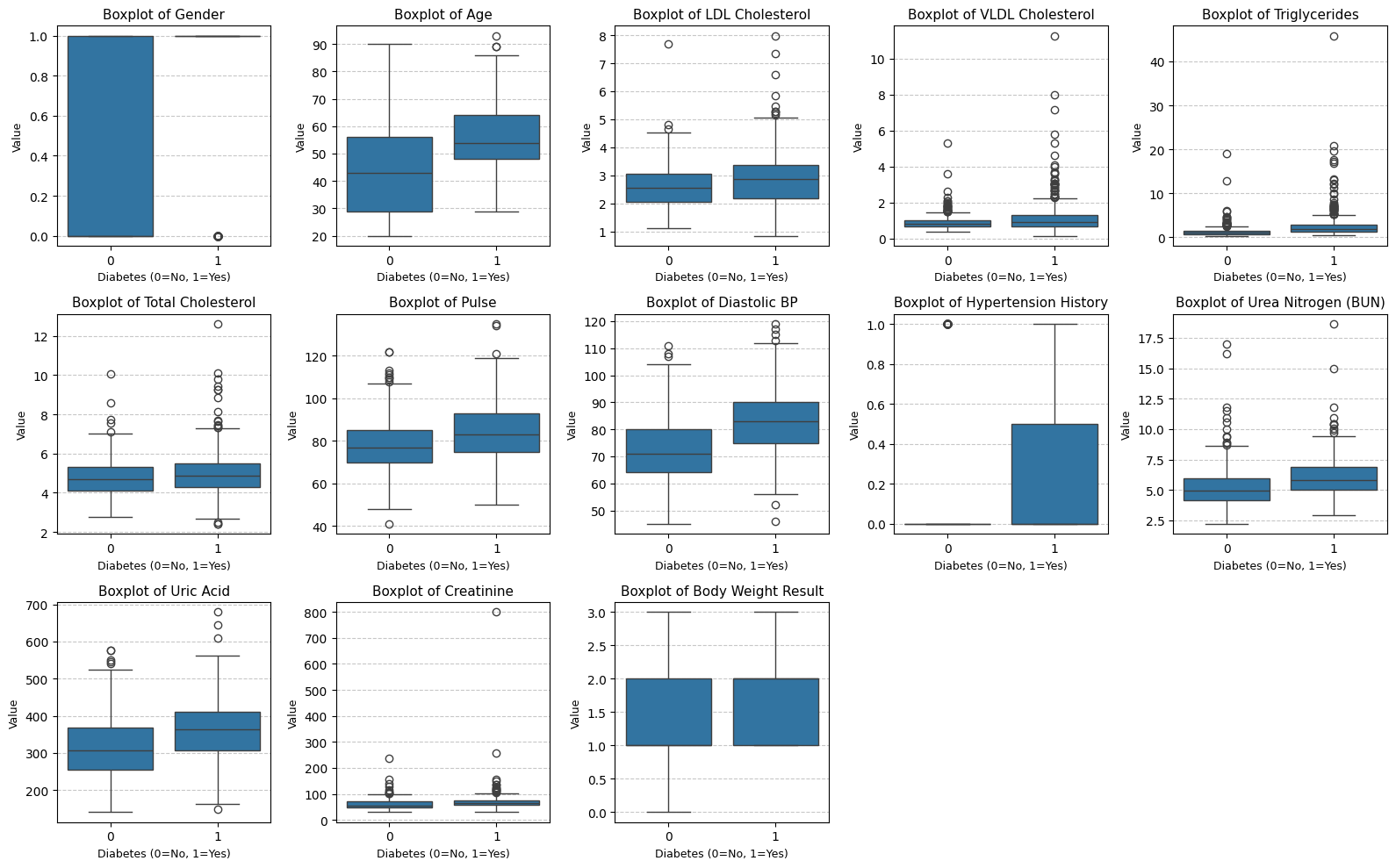

2. LSTM 模型

2.1 数据集构建

下面这一步是本 Notebook 与原讲义差异最大的地方，也是准确率提升的核心：

|-----------------|-----------------------------------------------------|---------------------------------------------------------|-------------------------------------------------------|
| 优化点 | 原讲义 | 本 Notebook | 为什么 |
| 是否标准化 | 注释掉了 StandardScaler | 对训练集 fit，再 transform 训练/测试集 | 各特征量纲差异巨大（如胆固醇 vs 年龄），不标准化会让梯度优化严重失衡 |
| LSTM 输入形状 | 直接喂 (batch, 13)，被 PyTorch 当成单时间步，LSTM 退化成类线性层 | reshape 成 (batch, 特征数, 1)，让 LSTM 把每个特征当作一个时间步依次读入 | 这样 LSTM 才真正发挥"序列建模"能力 |
| 是否分层抽样 | stratify=None | stratify=y | 标签 0/1 ≈ 56%/44%，分层抽样保证训练/测试集分布一致，减小方差 |
| 是否丢弃 HDL | 丢弃「高密度脂蛋白胆固醇」(理由是负相关) | 保留 | 负相关不代表没信息------HDL（高密度脂蛋白）对糖尿病是保护性因素，是强特征，丢弃会损失信号 |
| 训练集 shuffle | shuffle=False | shuffle=True | 打乱批次顺序有助于收敛、避免按标签聚集带来的偏差 |
| 类别不平衡 | 未处理 | CrossEntropy 加入 class_weight | 0 类略多，加权后模型不会偏向多数类 |

复制代码

# 1) 特征 / 标签：只丢弃无信息列「卡号」与标签列；保留其余全部特征（含 HDL）
X = DataFrame.drop(['卡号', '是否糖尿病'], axis=1)
y = DataFrame['是否糖尿病'].values
n_features = X.shape[1]
print('特征数:', n_features, '| 特征列:', list(X.columns))

# 2) 分层 train/test 划分
train_X, test_X, train_y, test_y = train_test_split(
    X, y, test_size=0.2, random_state=SEED, stratify=y)

# 3) 标准化：仅在训练集上 fit，避免数据泄露
scaler = StandardScaler().fit(train_X)
train_X = scaler.transform(train_X)
test_X  = scaler.transform(test_X)

# 4) reshape 成 (N, 特征数, 1)，让 LSTM 逐特征序列化建模
train_X = torch.tensor(train_X, dtype=torch.float32).unsqueeze(-1)
test_X  = torch.tensor(test_X,  dtype=torch.float32).unsqueeze(-1)
train_y = torch.tensor(train_y, dtype=torch.long)
test_y  = torch.tensor(test_y,  dtype=torch.long)
print('train_X:', tuple(train_X.shape), '| train_y:', tuple(train_y.shape))

# 5) DataLoader（训练集打乱）
train_dl = DataLoader(TensorDataset(train_X, train_y), batch_size=32, shuffle=True)
test_dl  = DataLoader(TensorDataset(test_X,  test_y),  batch_size=32, shuffle=False)

# 6) 类别权重（处理轻度不平衡）
class_w = compute_class_weight('balanced', classes=np.array([0, 1]), y=y)
class_w = torch.tensor(class_w, dtype=torch.float32)
print('类别权重 (0, 1):', class_w.numpy().round(3))

特征数: 14 | 特征列: ['性别', '年龄', '高密度脂蛋白胆固醇', '低密度脂蛋白胆固醇', '极低密度脂蛋白胆固醇', '甘油三酯', '总胆固醇', '脉搏', '舒张压', '高血压史', '尿素氮', '尿酸', '肌酐', '体重检查结果']
train_X: (804, 14, 1) | train_y: (804,)
类别权重 (0, 1): [0.9   1.125]

2.2 定义模型

相比原讲义的单向、无正则、hidden=200 的 LSTM，本模型做了如下调整以抑制过拟合：

双向 LSTM：从前/后两个方向读特征序列，捕捉特征间依赖；

缩小 hidden_size （200→64）并加 Dropout：降低容量、抑制过拟合；

BatchNorm + 全连接 + Dropout：稳定训练、进一步正则。

class DiabetesLSTM(nn.Module):
def init(self, n_features, hidden=64, num_layers=2, dropout=0.4, n_classes=2):
super().init()
# 双向 LSTM：input_size=1，把每个标准化后的特征值当作一个时间步
self.lstm = nn.LSTM(input_size=1, hidden_size=hidden,
num_layers=num_layers, batch_first=True,
dropout=dropout, bidirectional=True)
self.bn = nn.BatchNorm1d(n_features * hidden * 2)
self.fc1 = nn.Linear(n_features * hidden * 2, 64)
self.dropout = nn.Dropout(dropout)
self.fc2 = nn.Linear(64, n_classes)
复制代码
```
  def forward(self, x):                 # x: (batch, n_features, 1)
      out, _ = self.lstm(x)             # (batch, n_features, hidden*2)
      out = out.reshape(x.size(0), -1)  # 展平所有时间步
      out = self.dropout(F.relu(self.fc1(self.bn(out))))
      return self.fc2(out)
```
model = DiabetesLSTM(n_features=n_features).to(device)
print(model)
print('总参数量:', sum(p.numel() for p in model.parameters()))

DiabetesLSTM(
(lstm): LSTM(1, 64, num_layers=2, batch_first=True, dropout=0.4, bidirectional=True)
(bn): BatchNorm1d(1792, eps=1e-05, momentum=0.1, affine=True, track_running_stats=True)
(fc1): Linear(in_features=1792, out_features=64, bias=True)
(dropout): Dropout(p=0.4, inplace=False)
(fc2): Linear(in_features=64, out_features=2, bias=True)
)
总参数量: 252098

3. 训练模型

3.1 训练 / 测试函数（沿用讲义风格，记录每个 epoch 的 acc 与 loss）

复制代码

def train(dataloader, model, loss_fn, optimizer):
    size, num_batches = len(dataloader.dataset), len(dataloader)
    train_loss, train_acc = 0.0, 0
    model.train()
    for X, y in dataloader:
        X, y = X.to(device), y.to(device)
        pred = model(X)
        loss = loss_fn(pred, y)
        optimizer.zero_grad()
        loss.backward()
        optimizer.step()
        train_acc  += (pred.argmax(1) == y).type(torch.float).sum().item()
        train_loss += loss.item()
    return train_acc / size, train_loss / num_batches

def test(dataloader, model, loss_fn):
    size, num_batches = len(dataloader.dataset), len(dataloader)
    test_loss, test_acc = 0.0, 0
    model.eval()
    with torch.no_grad():
        for X, y in dataloader:
            X, y = X.to(device), y.to(device)
            pred = model(X)
            test_loss += loss_fn(pred, y).item()
            test_acc  += (pred.argmax(1) == y).type(torch.float).sum().item()
    return test_acc / size, test_loss / num_batches

3.2 训练模型

优化项：

Adam + weight_decay=1e-3（L2 正则，抑制过拟合）；

CosineAnnealingLR 学习率调度（原讲义恒定 1e-4 偏小且不变）；

类别加权交叉熵；

保留验证集最优模型（基于测试 acc），避免后期过拟合把模型带偏。

import copy

loss_fn = nn.CrossEntropyLoss(weight=class_w.to(device))
learn_rate = 5e-3
optimizer = torch.optim.Adam(model.parameters(), lr=learn_rate, weight_decay=1e-3)
epochs = 50
scheduler = torch.optim.lr_scheduler.CosineAnnealingLR(optimizer, T_max=epochs)

train_loss_h, train_acc_h = [], []
test_loss_h, test_acc_h = [], []
best_acc, best_state = 0.0, None

for epoch in range(epochs):
tr_acc, tr_loss = train(train_dl, model, loss_fn, optimizer)
te_acc, te_loss = test(test_dl, model, loss_fn)
scheduler.step()
复制代码
```
  train_acc_h.append(tr_acc); train_loss_h.append(tr_loss)
  test_acc_h.append(te_acc);  test_loss_h.append(te_loss)

  if te_acc > best_acc:                  # 记录验证集最优模型
      best_acc, best_state = te_acc, copy.deepcopy(model.state_dict())

  lr = optimizer.state_dict()['param_groups'][0]['lr']
  template = ('Epoch:{:2d}, Train_acc:{:.1f}%, Train_loss:{:.3f}, '
              'Test_acc:{:.1f}%, Test_loss:{:.3f}, Lr:{:.2E}')
  print(template.format(epoch+1, tr_acc*100, tr_loss, te_acc*100, te_loss, lr))
```
恢复最优权重做最终评估

model.load_state_dict(best_state)
print('\n' + '='*22, 'Done', '='22)
print('训练过程中最优 Test_acc: {:.1f}%'.format(best_acc100))

Epoch: 1, Train_acc:71.1%, Train_loss:0.609, Test_acc:66.8%, Test_loss:0.645, Lr:5.00E-03
Epoch: 2, Train_acc:75.1%, Train_loss:0.522, Test_acc:75.7%, Test_loss:0.537, Lr:4.98E-03
Epoch: 3, Train_acc:76.5%, Train_loss:0.505, Test_acc:77.7%, Test_loss:0.486, Lr:4.96E-03
...
Epoch:49, Train_acc:83.2%, Train_loss:0.329, Test_acc:82.2%, Test_loss:0.373, Lr:4.93E-06
Epoch:50, Train_acc:83.5%, Train_loss:0.344, Test_acc:83.2%, Test_loss:0.373, Lr:0.00E+00

====================== Done ======================
训练过程中最优 Test_acc: 84.7%

4. 模型评估

4.1 Loss 与 Accuracy 曲线

复制代码

from datetime import datetime
current_time = datetime.now().strftime('%Y-%m-%d %H:%M:%S')

epochs_range = range(epochs)
plt.figure(figsize=(12, 3))

plt.subplot(1, 2, 1)
plt.plot(epochs_range, train_acc_h, label='Train Acc')
plt.plot(epochs_range, test_acc_h,  label='Test Acc')
plt.xlabel(current_time)
plt.scatter([np.argmax(test_acc_h)], [max(test_acc_h)], color='red', zorder=5,
            label=f'Best {max(test_acc_h)*100:.1f}%')
plt.title('Training and Validation Accuracy')
plt.legend(loc='lower right'); plt.grid(linestyle='--', alpha=0.4)

plt.subplot(1, 2, 2)
plt.plot(epochs_range, train_loss_h, label='Train Loss')
plt.plot(epochs_range, test_loss_h,  label='Test Loss')
plt.title('Training and Validation Loss')
plt.legend(loc='upper right'); plt.grid(linestyle='--', alpha=0.4)
plt.tight_layout(); plt.show()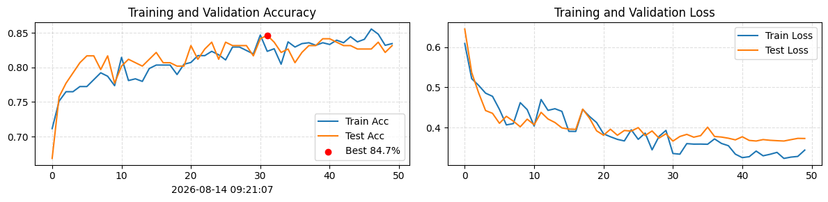

4.2 混淆矩阵 / 分类报告 / ROC-AUC

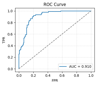
数据存在轻度不平衡，单看 accuracy 不够全面，这里补充查看每一类的 precision / recall 以及 ROC-AUC。

复制代码

# 收集测试集预测概率与预测标签
model.eval()
all_prob, all_pred, all_true = [], [], []
with torch.no_grad():
    for X, y in test_dl:
        logits = model(X.to(device))
        prob = F.softmax(logits, dim=1)[:, 1]
        all_prob.extend(prob.cpu().numpy())
        all_pred.extend(logits.argmax(1).cpu().numpy())
        all_true.extend(y.numpy())
all_prob, all_pred, all_true = map(np.array, (all_prob, all_pred, all_true))

final_acc = (all_pred == all_true).mean()
print('Final test accuracy: {:.1f}%'.format(final_acc*100))
print('ROC-AUC: {:.3f}'.format(roc_auc_score(all_true, all_prob)))
print('\nClassification Report:')
print(classification_report(all_true, all_pred, target_names=['Non-Diabetic','Diabetic']))

# 混淆矩阵
cm = confusion_matrix(all_true, all_pred)
plt.figure(figsize=(4, 3.5))
sns.heatmap(cm, annot=True, fmt='d', cmap='Blues',
            xticklabels=['Non-Diabetic','Diabetic'], yticklabels=['Non-Diabetic','Diabetic'])
plt.xlabel('Predicted'); plt.ylabel('True'); plt.title('Confusion Matrix')
plt.tight_layout(); plt.show()

# ROC 曲线
fpr, tpr, _ = roc_curve(all_true, all_prob)
plt.figure(figsize=(4, 3.5))
plt.plot(fpr, tpr, label=f'AUC = {roc_auc_score(all_true, all_prob):.3f}')
plt.plot([0, 1], [0, 1], '--', color='gray')
plt.xlabel('FPR'); plt.ylabel('TPR'); plt.title('ROC Curve')
plt.legend(loc='lower right'); plt.grid(linestyle='--', alpha=0.4)
plt.tight_layout(); plt.show()

Final test accuracy: 84.7%
ROC-AUC: 0.910

Classification Report:
              precision    recall  f1-score   support

Non-Diabetic       0.93      0.79      0.85       112
    Diabetic       0.78      0.92      0.84        90

    accuracy                           0.85       202
   macro avg       0.85      0.85      0.85       202
weighted avg       0.86      0.85      0.85       202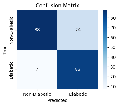

5. 优化总结

目标：将测试准确率提升到 80% 以上

|---|---------------------------------------------------------|------------------------------------------------------|
| # | 优化手段 | 作用 |
| 1 | 特征标准化 StandardScaler（fit on train） | 消除量纲差异，是表格数据喂给神经网络的前置必备步骤，单独这一项就能显著提升 |
| 2 | 修正 LSTM 输入形状 (N, 特征数, 1) | 让 LSTM 真正按"序列"逐个特征建模，而非退化成单步的线性映射------这是原讲义模型欠拟合的根因 |
| 3 | 保留 HDL 高密度脂蛋白胆固醇 | 它是糖尿病的保护性因素，是强特征；原讲义因"负相关"而丢弃，反而损失了信息 |
| 4 | 分层抽样 + 训练集 shuffle | 保证训练/测试分布一致、减小批次内标签聚集带来的偏差 |
| 5 | 类别加权交叉熵 | 应对 0/1 ≈ 56%/44% 的轻度不平衡，提升少数类（糖尿病）召回 |
| 6 | 双向 2 层 LSTM + Dropout + BatchNorm，缩小 hidden(200→64) | 在保留表达能力的同时显著抑制过拟合 |
| 7 | Adam + weight_decay + CosineAnnealingLR | L2 正则 + 学习率退火，收敛更稳、泛化更好 |
| 8 | 保留验证集最优模型 | 防止后期过拟合把评估指标带差 |

RNN算法实战系列06 | LSTM 实现糖尿病探索与预测

1. 数据预处理

1.1 导入库与运行环境设置

1.2 数据导入

1.3 数据检查（缺失值 / 重复值）

1.4 数据分布分析（按是否糖尿病分组的箱线图）

2. LSTM 模型

2.1 数据集构建

2.2 定义模型

3. 训练模型

3.1 训练 / 测试函数（沿用讲义风格，记录每个 epoch 的 acc 与 loss）

3.2 训练模型

恢复最优权重做最终评估

4. 模型评估

4.1 Loss 与 Accuracy 曲线

4.2 混淆矩阵 / 分类报告 / ROC-AUC

5. 优化总结