Transformer 训练资源估算：以 CS336 GPT-2 XL 配置为例

本文以 CS336 作业中的 GPT-2 XL 配置为例，估算 Transformer 训练过程中的显存、FLOPs 和训练时间。

本文使用的模型配置如下：

参数	符号	数值
词表大小	V V V	50257
上下文长度	T T T	1024
Transformer 层数	L L L	48
隐藏维度	d d d	1600
注意力头数	H H H	25
FFN 隐藏维度	d f f d_{\mathrm{ff}} dff	4288

这里的模型结构是 CS336 实现中的结构：

Token Embedding；
多头注意力；
SwiGLU；
RMSNorm；
最后的语言模型输出层；
Embedding 和 lm_head 不共享参数；
使用 FP32 进行估算。

注意：这更准确地说是"GPT-2 XL 尺寸的 CS336 Transformer"，并不是原始 GPT-2 XL 的完全相同实现。CS336 使用了 RoPE、RMSNorm 和 SwiGLU。

一、FP32 训练显存由哪些部分组成？

训练时显存主要由四部分组成：

M t o t a l = M p a r a m + M g r a d + M o p t i m i z e r + M a c t i v a t i o n M_{\mathrm{total}}=M_{\mathrm{param}}+M_{\mathrm{grad}}+M_{\mathrm{optimizer}}+M_{\mathrm{activation}} Mtotal=Mparam+Mgrad+Moptimizer+Mactivation

分别是：

模型参数；
参数梯度；
优化器状态；
前向传播中保存的激活值。

1. 模型参数显存

先计算模型参数量。

Embedding 和 lm_head 各有一个矩阵：

P e m b e d d i n g = V d P_{\mathrm{embedding}}=Vd Pembedding=Vd

P l m _ h e a d = V d P_{\mathrm{lm\_head}}=Vd Plm_head=Vd

所以两者合计：

P v o c a b = 2 V d P_{\mathrm{vocab}}=2Vd Pvocab=2Vd

每个 Transformer 层包含：

注意力的 Q , K , V , O Q,K,V,O Q,K,V,O 四个线性层：

P a t t e n t i o n = 4 d 2 P_{\mathrm{attention}}=4d^2 Pattention=4d2

SwiGLU 的 w 1 , w 2 , w 3 w_1,w_2,w_3 w1,w2,w3 三个线性层：

P S w i G L U = 3 d d f f P_{\mathrm{SwiGLU}}=3dd_{\mathrm{ff}} PSwiGLU=3ddff

两个 RMSNorm：

P n o r m = 2 d P_{\mathrm{norm}}=2d Pnorm=2d

因此总参数量为：

P = 2 V d + L ( 4 d 2 + 3 d d f f + 2 d ) + d P=2Vd+L(4d^2+3dd_{\mathrm{ff}}+2d)+d P=2Vd+L(4d2+3ddff+2d)+d

最后的 + d +d +d 是模型最后一个 RMSNorm 的参数。

代入数值：

P = 2 × 50257 × 1600 + 48 ( 4 × 1600 2 + 3 × 1600 × 4288 + 2 × 1600 ) + 1600 P=2\times50257\times1600+48(4\times1600^2+3\times1600\times4288+2\times1600)+1600 P=2×50257×1600+48(4×16002+3×1600×4288+2×1600)+1600

P = 1 , 640 , 452 , 800 P=1,640,452,800 P=1,640,452,800

所以模型大约有：

1.64 B 个参数 \boxed{1.64\text{B 个参数}} 1.64B 个参数

FP32 每个参数占 4 Bytes，因此：

M p a r a m = 4 P M_{\mathrm{param}}=4P Mparam=4P

M p a r a m = 6 , 561 , 811 , 200 Bytes ≈ 6.562 GB M_{\mathrm{param}}=6,561,811,200\text{ Bytes}\approx6.562\text{ GB} Mparam=6,561,811,200 Bytes≈6.562 GB

2. 梯度显存

每个参数通常对应一个同样大小的梯度张量：

M g r a d = 4 P M_{\mathrm{grad}}=4P Mgrad=4P

所以：

M g r a d ≈ 6.562 GB M_{\mathrm{grad}}\approx6.562\text{ GB} Mgrad≈6.562 GB

3. AdamW 优化器状态显存

AdamW 为每个参数保存两个状态：

一阶动量 m t m_t mt；
二阶动量 v t v_t vt。

它们的更新公式是：

m t = β 1 m t − 1 + ( 1 − β 1 ) g t m_t=\beta_1m_{t-1}+(1-\beta_1)g_t mt=β1mt−1+(1−β1)gt

v t = β 2 v t − 1 + ( 1 − β 2 ) g t 2 v_t=\beta_2v_{t-1}+(1-\beta_2)g_t^2 vt=β2vt−1+(1−β2)gt2

其中：

g t g_t gt 是当前梯度；
m t m_t mt 是梯度的一阶滑动平均；
v t v_t vt 是梯度平方的二阶滑动平均。

因为 m t m_t mt 和 v t v_t vt 都与参数形状相同，所以：

M m = 4 P M_m=4P Mm=4P

M v = 4 P M_v=4P Mv=4P

优化器状态总显存为：

M o p t i m i z e r = M m + M v = 8 P M_{\mathrm{optimizer}}=M_m+M_v=8P Moptimizer=Mm+Mv=8P

M o p t i m i z e r ≈ 13.123 GB M_{\mathrm{optimizer}}\approx13.123\text{ GB} Moptimizer≈13.123 GB

因此，暂时不考虑激活值时：

M f i x e d = 4 P + 4 P + 8 P = 16 P M_{\mathrm{fixed}}=4P+4P+8P=16P Mfixed=4P+4P+8P=16P

M f i x e d = 26 , 247 , 244 , 800 Bytes M_{\mathrm{fixed}}=26,247,244,800\text{ Bytes} Mfixed=26,247,244,800 Bytes

M f i x e d ≈ 26.247 GB \boxed{M_{\mathrm{fixed}}\approx26.247\text{ GB}} Mfixed≈26.247 GB

可以看到，AdamW 的两个状态一共占 8 P 8P 8P，再加上参数和梯度的 8 P 8P 8P，所以固定部分总共约为：

16 P \boxed{16P} 16P

二、激活值显存估算

激活值是前向传播过程中产生的中间张量。反向传播时需要使用它们计算梯度，因此不能全部立即释放。

设：

B B B：batch size；
T T T：序列长度；
d d d：隐藏维度；
H H H：注意力头数。

1. 注意力部分

输入经过三个线性层得到：

Q , K , V ∈ R B × T × d Q,K,V\in\mathbb{R}^{B\times T\times d} Q,K,V∈RB×T×d

它们一共需要：

3 B T d 3BTd 3BTd

注意力分数矩阵的形状是：

Q K ⊤ ∈ R B × H × T × T QK^\top\in\mathbb{R}^{B\times H\times T\times T} QK⊤∈RB×H×T×T

因此需要：

B H T 2 BHT^2 BHT2

softmax 的结果形状相同，还需要：

B H T 2 BHT^2 BHT2

注意力输出经过多头拼接后形状回到：

B × T × d B\times T\times d B×T×d

再加上输出投影结果，可以近似记为 2 B T d 2BTd 2BTd。

因此注意力部分的主要激活值数量近似为：

A a t t e n t i o n ≈ 5 B T d + 2 B H T 2 A_{\mathrm{attention}}\approx5BTd+2BHT^2 Aattention≈5BTd+2BHT2

2. SwiGLU 部分

SwiGLU 的公式为：

S w i G L U ( x ) = W 2 ( S i L U ( W 1 x ) ⊙ W 3 x ) \mathrm{SwiGLU}(x)=W_2\left(\mathrm{SiLU}(W_1x)\odot W_3x\right) SwiGLU(x)=W2(SiLU(W1x)⊙W3x)

其中：

W 1 x ∈ R B × T × d f f W_1x\in\mathbb{R}^{B\times T\times d_{\mathrm{ff}}} W1x∈RB×T×dff

W 3 x ∈ R B × T × d f f W_3x\in\mathbb{R}^{B\times T\times d_{\mathrm{ff}}} W3x∈RB×T×dff

逐元素相乘后仍然是：

B × T × d f f B\times T\times d_{\mathrm{ff}} B×T×dff

按照需要保存的主要中间结果近似记账：

A S w i G L U ≈ 4 B T d f f + B T d A_{\mathrm{SwiGLU}}\approx4BTd_{\mathrm{ff}}+BTd ASwiGLU≈4BTdff+BTd

3. 单层激活值近似

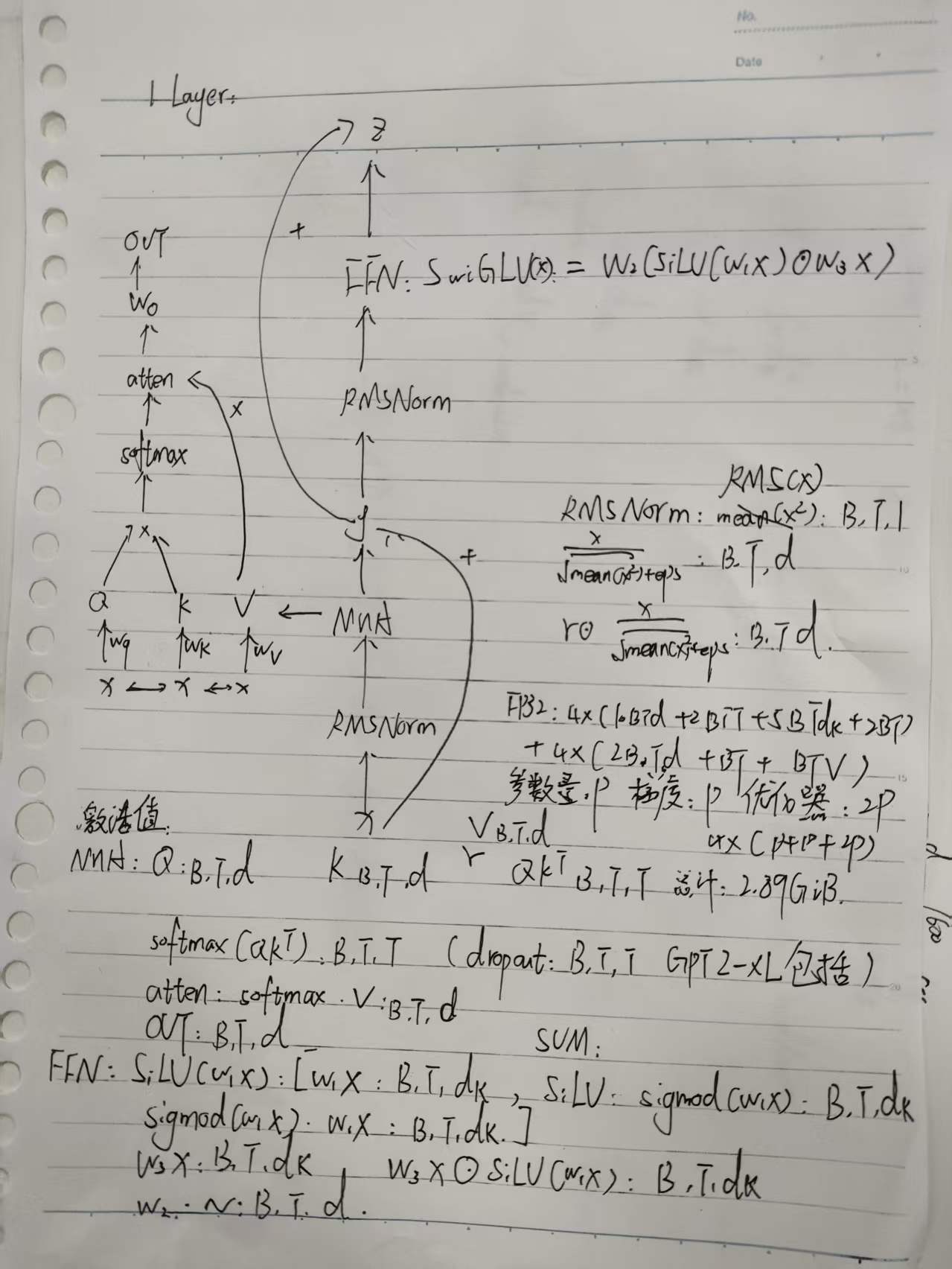
结合注意力、RMSNorm、残差连接和 SwiGLU，按照手写草稿中的合并口径，单层可以近似写为：

A l a y e r ≈ 9 B T d + 4 B T d f f + 2 B H T 2 A_{\mathrm{layer}}\approx9BTd+4BTd_{\mathrm{ff}}+2BHT^2 Alayer≈9BTd+4BTdff+2BHT2

整个模型的激活值数量近似为：

A ( B ) ≈ 2 B T d + L ( 9 B T d + 4 B T d f f + 2 B H T 2 ) + B T V A(B)\approx2BTd+L(9BTd+4BTd_{\mathrm{ff}}+2BHT^2)+BTV A(B)≈2BTd+L(9BTd+4BTdff+2BHT2)+BTV

其中：

2 B T d 2BTd 2BTd 表示输入和最终隐藏状态等主要张量；
L ( ⋯ ) L(\cdots) L(⋯) 表示所有 Transformer 层；
B T V BTV BTV 表示最后输出的 logits。

FP32 每个元素占 4 Bytes，因此：

M a c t i v a t i o n ( B ) = 4 A ( B ) M_{\mathrm{activation}}(B)=4A(B) Mactivation(B)=4A(B)

手写推导图

手写激活值显存推导：

4. 代入具体参数

代入：

T = 1024 , d = 1600 , L = 48 , H = 25 , d f f = 4288 , V = 50257 T=1024,\quad d=1600,\quad L=48,\quad H=25,\quad d_{\mathrm{ff}}=4288,\quad V=50257 T=1024,d=1600,L=48,H=25,dff=4288,V=50257

可得到：

M a c t i v a t i o n ( B ) = 16 , 488 , 665 , 088 B Bytes M_{\mathrm{activation}}(B)=16,488,665,088B\text{ Bytes} Mactivation(B)=16,488,665,088B Bytes

约为：

M a c t i v a t i o n ( B ) ≈ 16.489 B GB M_{\mathrm{activation}}(B)\approx16.489B\text{ GB} Mactivation(B)≈16.489B GB

因此总显存近似为：

M p e a k ( B ) = 26 , 247 , 244 , 800 + 16 , 488 , 665 , 088 B M_{\mathrm{peak}}(B)=26,247,244,800+16,488,665,088B Mpeak(B)=26,247,244,800+16,488,665,088B

换算成 GB：

M p e a k ( B ) ≈ 26.247 + 16.489 B GB \boxed{M_{\mathrm{peak}}(B)\approx26.247+16.489B\text{ GB}} Mpeak(B)≈26.247+16.489B GB

80GB 显存下：

B max ⁡ = ⌊ 80 − 26.247 16.489 ⌋ B_{\max}=\left\lfloor\frac{80-26.247}{16.489}\right\rfloor Bmax=⌊16.48980−26.247⌋

B max ⁡ = 3 B_{\max}=3 Bmax=3

检查：

M p e a k ( 3 ) ≈ 75.713 GB M_{\mathrm{peak}}(3)\approx75.713\text{ GB} Mpeak(3)≈75.713 GB

M p e a k ( 4 ) ≈ 92.202 GB M_{\mathrm{peak}}(4)\approx92.202\text{ GB} Mpeak(4)≈92.202 GB

所以按照这个激活值近似公式：

B max ⁡ = 3 \boxed{B_{\max}=3} Bmax=3

但是，这个公式没有完整计算：

PyTorch softmax 中的临时张量；
masked_fill 产生的临时结果；
CUDA caching allocator 的缓存；
其他运行时开销。

因此实际训练时建议保守使用：

text 复制代码

micro_batch_size = 2

三、单次训练 step 的 FLOPs

公式是：

( m × n ) ( n × p ) (m\times n)(n\times p) (m×n)(n×p)

需要进行 m n p mnp mnp 次乘法和大约 m n p mnp mnp 次加法，因此：

F m a t m u l ≈ 2 m n p F_{\mathrm{matmul}}\approx2mnp Fmatmul≈2mnp

1. 注意力投影

Q , K , V , O Q,K,V,O Q,K,V,O 一共四个线性层，每个线性层的 FLOPs 约为：

2 B T d 2 2BTd^2 2BTd2

四个线性层：

F p r o j e c t i o n = 8 B T d 2 F_{\mathrm{projection}}=8BTd^2 Fprojection=8BTd2

2. 注意力矩阵乘法

计算 Q K ⊤ QK^\top QK⊤：

F Q K ⊤ = 2 B H T 2 d h e a d F_{QK^\top}=2BHT^2d_{\mathrm{head}} FQK⊤=2BHT2dhead

由于：

d = H d h e a d d=Hd_{\mathrm{head}} d=Hdhead

所以：

F Q K ⊤ = 2 B T 2 d F_{QK^\top}=2BT^2d FQK⊤=2BT2d

计算注意力权重与 V V V 的乘法：

F A V = 2 B T 2 d F_{\mathrm{AV}}=2BT^2d FAV=2BT2d

两者合计：

F a t t e n t i o n = 4 B T 2 d F_{\mathrm{attention}}=4BT^2d Fattention=4BT2d

3. SwiGLU

SwiGLU 有三个线性层：

W 1 , W 2 , W 3 W_1,\quad W_2,\quad W_3 W1,W2,W3

每个相关矩阵乘法的 FLOPs 约为：

2 B T d d f f 2BTdd_{\mathrm{ff}} 2BTddff

所以：

F S w i G L U = 6 B T d d f f F_{\mathrm{SwiGLU}}=6BTdd_{\mathrm{ff}} FSwiGLU=6BTddff

4. 语言模型输出层

最后的 lm_head 将隐藏维度 d d d 映射到词表大小 V V V：

F l m _ h e a d = 2 B T d V F_{\mathrm{lm\_head}}=2BTdV Flm_head=2BTdV

5. 总前向 FLOPs

因此：

F f o r w a r d = L ( 8 B T d 2 + 4 B T 2 d + 6 B T d d f f ) + 2 B T d V F_{\mathrm{forward}}=L(8BTd^2+4BT^2d+6BTdd_{\mathrm{ff}})+2BTdV Fforward=L(8BTd2+4BT2d+6BTddff)+2BTdV

四、AdamW 参数更新的 FLOPs

AdamW 的完整更新公式为：

m t = β 1 m t − 1 + ( 1 − β 1 ) g t m_t=\beta_1m_{t-1}+(1-\beta_1)g_t mt=β1mt−1+(1−β1)gt

v t = β 2 v t − 1 + ( 1 − β 2 ) g t 2 v_t=\beta_2v_{t-1}+(1-\beta_2)g_t^2 vt=β2vt−1+(1−β2)gt2

偏差修正：

m ^ t = m t 1 − β 1 t \hat m_t=\frac{m_t}{1-\beta_1^t} m^t=1−β1tmt

v ^ t = v t 1 − β 2 t \hat v_t=\frac{v_t}{1-\beta_2^t} v^t=1−β2tvt

AdamW 的参数更新为：

θ t = ( 1 − η λ ) θ t − 1 − η m ^ t v ^ t + ϵ \theta_t=(1-\eta\lambda)\theta_{t-1}-\eta\frac{\hat m_t}{\sqrt{\hat v_t}+\epsilon} θt=(1−ηλ)θt−1−ηv^t +ϵm^t

其中：

θ \theta θ：模型参数；
η \eta η：学习率；
λ \lambda λ：weight decay；
m t m_t mt：一阶动量；
v t v_t vt：二阶动量；
ϵ \epsilon ϵ：防止除零的小常数。

对每一个参数，粗略计算：

操作	近似 FLOPs
更新 m t m_t mt	3
更新 v t v_t vt	4
偏差修正	2
开方、加 epsilon、除法	3
权重衰减和参数更新	3

所以可以近似写成：

F A d a m W ≈ 15 P F_{\mathrm{AdamW}}\approx15P FAdamW≈15P

实际实现中，一些标量计算可以预先合并或融合，因此工程估算中也经常使用：

F A d a m W ≈ 12 P F_{\mathrm{AdamW}}\approx12P FAdamW≈12P

本文采用简化估算：

F A d a m W ≈ 12 P F_{\mathrm{AdamW}}\approx12P FAdamW≈12P

因此，一次完整训练 step 的 FLOPs 为：

F s t e p = F f o r w a r d + F b a c k w a r d + F A d a m W F_{\mathrm{step}}=F_{\mathrm{forward}}+F_{\mathrm{backward}}+F_{\mathrm{AdamW}} Fstep=Fforward+Fbackward+FAdamW

题目给出：

F f o r w a r d : F b a c k w a r d = 1 : 2 F_{\mathrm{forward}}:F_{\mathrm{backward}}=1:2 Fforward:Fbackward=1:2

所以：

F b a c k w a r d = 2 F f o r w a r d F_{\mathrm{backward}}=2F_{\mathrm{forward}} Fbackward=2Fforward

最终：

F s t e p ≈ 3 F f o r w a r d + 12 P \boxed{F_{\mathrm{step}}\approx3F_{\mathrm{forward}}+12P} Fstep≈3Fforward+12P

这里的 12 P 12P 12P 就是 AdamW 参数更新的近似 FLOPs。

五、训练 40 万步需要多长时间？

题目给出：

H100 FP32 峰值算力：495 TFLOPS；
MFU：50%；
训练步数：400000；
有效 batch size：1024。

1. H100 的有效算力

MFU 表示实际达到理论峰值的比例：

F e f f e c t i v e = 495 × 10 12 × 50 % F_{\mathrm{effective}}=495\times10^{12}\times50\% Feffective=495×1012×50%

F e f f e c t i v e = 247.5 × 10 12 FLOPs/s F_{\mathrm{effective}}=247.5\times10^{12}\text{ FLOPs/s} Feffective=247.5×1012 FLOPs/s

2. 每一步的 FLOPs

代入 B = 1024 B=1024 B=1024：

F f o r w a r d ≈ 3.60117 × 10 15 F_{\mathrm{forward}}\approx3.60117\times10^{15} Fforward≈3.60117×1015

AdamW 更新：

F A d a m W ≈ 12 P ≈ 1.9685 × 10 10 F_{\mathrm{AdamW}}\approx12P\approx1.9685\times10^{10} FAdamW≈12P≈1.9685×1010

所以：

F s t e p ≈ 3 ( 3.60117 × 10 15 ) + 1.9685 × 10 10 F_{\mathrm{step}}\approx3(3.60117\times10^{15})+1.9685\times10^{10} Fstep≈3(3.60117×1015)+1.9685×1010

F s t e p ≈ 1.08035 × 10 16 FLOPs F_{\mathrm{step}}\approx1.08035\times10^{16}\text{ FLOPs} Fstep≈1.08035×1016 FLOPs

3. 总 FLOPs

F t o t a l = 400000 F s t e p F_{\mathrm{total}}=400000F_{\mathrm{step}} Ftotal=400000Fstep

F t o t a l ≈ 4.32141 × 10 21 FLOPs F_{\mathrm{total}}\approx4.32141\times10^{21}\text{ FLOPs} Ftotal≈4.32141×1021 FLOPs

4. 总训练时间

t = F t o t a l F e f f e c t i v e t=\frac{F_{\mathrm{total}}}{F_{\mathrm{effective}}} t=FeffectiveFtotal

t = 4.32141 × 10 21 247.5 × 10 12 t=\frac{4.32141\times10^{21}}{247.5\times10^{12}} t=247.5×10124.32141×1021

t ≈ 17 , 460 , 261 秒 t\approx17,460,261\text{ 秒} t≈17,460,261 秒

换算为小时：

t h o u r s = 17 , 460 , 261 3600 t_{\mathrm{hours}}=\frac{17,460,261}{3600} thours=360017,460,261

t ≈ 4850.1 小时 \boxed{t\approx4850.1\text{ 小时}} t≈4850.1 小时

换算为天：

t ≈ 202.1 天 \boxed{t\approx202.1\text{ 天}} t≈202.1 天

这个结果是理想化估算，没有计算：

数据读取时间；
通信时间；
checkpoint 保存时间；
验证过程；
CUDA kernel 启动开销；
GPU 利用率波动。

六、物理 batch size 与有效 batch size

80GB 显存无法直接放下 batch_size=1024。

如果实际显存只能容纳：

text 复制代码

micro_batch_size = 2

那么可以使用梯度累积：

B e f f e c t i v e = B m i c r o × N a c c u m u l a t i o n B_{\mathrm{effective}}=B_{\mathrm{micro}}\times N_{\mathrm{accumulation}} Beffective=Bmicro×Naccumulation

令有效 batch size 为 1024：

1024 = 2 × 512 1024=2\times512 1024=2×512

因此：

text 复制代码

micro_batch_size = 2
gradient_accumulation_steps = 512
effective_batch_size = 1024

训练伪代码：

python 复制代码

optimizer.zero_grad()

for _ in range(512):
    logits = model(x)
    loss = cross_entropy(logits, targets)

    # 避免累积后的梯度放大 512 倍
    loss = loss / 512
    loss.backward()

optimizer.step()

这里要区分：

micro_batch_size=2：一次实际放入显存的 batch；
effective_batch_size=1024：累计 512 次后，相当于一次更新使用的样本数；
optimizer.step()：每累计 512 个 micro-batch 执行一次。

理论上，梯度累积不会改变这 1024 个样本对应的总 FLOPs，只是把一次大 batch 拆成了多次小 batch 执行。

七、源代码

本文涉及的模型、交叉熵、AdamW、梯度裁剪、学习率调度和训练脚本代码可以在这里查看：

GitHub 源代码：assignment1-basics-main

本文中的激活值显存公式采用的是手算近似，用于理解显存随 batch size、序列长度和模型结构变化的规律。实际 PyTorch 运行时显存可能更高，最终应以显存监控工具的实际结果为准。