CMA-Former：基于级联多头注意力 Transformer 的 DOA 波达方向估计（PyTorch 实现）

本文环境：Python 3.9 + PyTorch 1.12 + CUDA 11.3 + Tesla V100（消费级 GPU 亦可运行，显存占用仅 1.6GB）

摘要

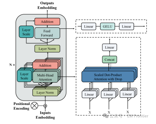
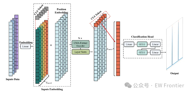
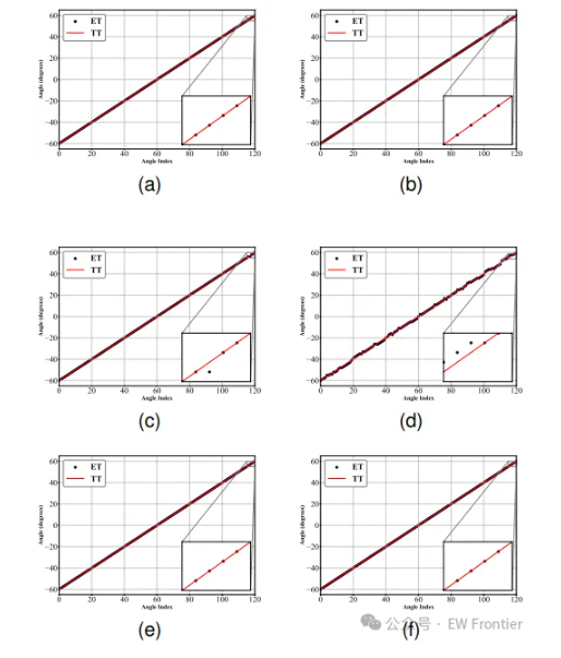
针对传统子空间类 DOA 估计算法（MUSIC/ESPRIT）在低信噪比下性能退化、依赖信源数先验的问题，本文实现 CMA-Former ：将 DOA 估计建模为 121 类多标签分类，输入为协方差矩阵上三角非对角元素的 4 维混合表征（实部/虚部/sin 相位/cos 相位），核心编码器在每个 Block 内串行级联 4/8/16 头注意力 ，辅以 LayerScale、随机深度与 CLS token 池化。实验表明：16 元均匀线阵在 -16dB 下三源 RMSE 达 0.475° （MUSIC 为 12.67°），模型仅 1.57M 参数 、单次推理 1.64ms 。

1. 问题定义

角度网格：-60° ~ 60°，步长 1°，共 121 类；
标签：多标签 one-hot（多源时为 multi-hot），训练时可采用高斯软标签（σ=2°）抑制网格边界震荡；
输入：16 元均匀线阵（d=λ/2），快照 1000，由接收信号协方差矩阵提取上三角非对角元素，共 120 个复数 token。

1.1 仿真数据生成（供参考）

python 复制代码

import numpy as np

def generate_steering_vector(theta, N=16, d=0.5):
    """均匀线阵导向矢量：a(theta) = exp(j*2π*d*n*sinθ)"""
    return np.exp(1j * 2 * np.pi * d * np.arange(N) * np.sin(np.deg2rad(theta)))

def generate_received_signal(thetas, SNR, S, N=16, seed=None):
    """生成接收信号 X (N x S)
    Args:
        thetas: 来波角度列表（度），支持多源
        SNR: 信噪比(dB)
        S: 快照数
    """
    if seed is not None:
        np.random.seed(seed)
    A = np.column_stack([generate_steering_vector(t, N) for t in thetas])
    K = len(thetas)
    signal = (np.random.randn(K, S) + 1j * np.random.randn(K, S)) / np.sqrt(2)   # 单位功率信号
    noise_power = 10 ** (-SNR / 10)
    noise = np.sqrt(noise_power / 2) * (np.random.randn(N, S) + 1j * np.random.randn(N, S))
    return A @ signal + noise          # X = A·s + n

数据生成要点：单/双/三源组合按类均衡采样；SNR 在 $-20, 0$ dB 内等间隔取值；标签在 -60°~60° 网格上打 multi-hot（或高斯软标签）。

2. 数据特征提取

协方差矩阵共轭对称，故仅取上三角；相位是 DOA 的核心载体，故显式拼接 sin/cos 分量：

python 复制代码

import numpy as np

def signal_to_network_input(X, N=16):
    """接收信号 X (N x snapshots) -> 网络输入 (120, 4)

    Args:
        X: 复接收信号矩阵, shape (N, snapshots)
        N: 阵元数
    Returns:
        r: 特征张量, shape (120, 4), 每行 = [real, imag, sin(phase), cos(phase)]
    """
    R = (X @ X.conj().T) / X.shape[1]          # 样本协方差矩阵 (N, N)

    # 上三角非对角元素（按行优先）
    r_cplx = np.array([R[i, j] for i in range(N) for j in range(i + 1, N)])

    # 4 维混合表征
    r = np.stack([
        r_cplx.real,                          # 实部
        r_cplx.imag,                          # 虚部
        np.sin(np.angle(r_cplx)),             # 相位正弦
        np.cos(np.angle(r_cplx)),             # 相位余弦
    ], axis=-1)
    return r

2.1 MUSIC 基线实现（用于对比）

python 复制代码

def music_spectrum(X, num_sources, theta_grid, d=0.5):
    """MUSIC 空间谱：1 / a^H·En·En^H·a
    Args:
        X: 接收信号 (N, snapshots)
        num_sources: 信源数（需要先验！）
        theta_grid: 角度搜索网格（度）
    """
    M, S = X.shape
    R = (X @ X.conj().T) / S                          # 协方差矩阵
    eigvals, eigvecs = np.linalg.eigh(R)
    eigvecs = eigvecs[:, np.argsort(eigvals)[::-1]]   # 特征向量按特征值降序
    En = eigvecs[:, num_sources:]                     # 噪声子空间（后 M-K 列）
    spectrum = np.zeros(len(theta_grid))
    for i, th in enumerate(theta_grid):
        a = np.exp(1j * 2 * np.pi * d * np.sin(np.deg2rad(th)) * np.arange(M))
        spectrum[i] = 1.0 / (np.abs(a.conj() @ En @ En.conj() @ a) + 1e-12)
    return spectrum / spectrum.max()

注意 MUSIC 需要提前给定信源数 num_sources，这正是它工程落地的主要障碍之一；而 CMA-Former 通过多标签分类天然支持未知信源数场景。

3. 模型定义：CMA-Former

3.1 基础模块

python 复制代码

import torch
import torch.nn as nn

class DropPath(nn.Module):
    """随机深度（Stochastic Depth），推理时为恒等映射"""
    def __init__(self, drop_prob=0.0):
        super().__init__()
        self.drop_prob = drop_prob

    def forward(self, x):
        if self.drop_prob == 0.0 or not self.training:
            return x
        keep = 1 - self.drop_prob
        mask = torch.rand(x.shape[0], 1, 1, device=x.device) < keep
        return x * mask.to(x.dtype) / keep

class LayerScale(nn.Module):
    """逐通道可学习缩放，初始值很小，稳定深层训练"""
    def __init__(self, dim, init_values=1e-4):
        super().__init__()
        self.gamma = nn.Parameter(init_values * torch.ones(dim))

    def forward(self, x):
        return self.gamma * x

class MSA(nn.Module):
    """多头自注意力"""
    def __init__(self, dim, num_heads=8, qkv_bias=True):
        super().__init__()
        self.num_heads = num_heads
        head_dim = dim // num_heads
        self.scale = head_dim ** -0.5
        self.qkv = nn.Linear(dim, dim * 3, bias=qkv_bias)
        self.proj = nn.Linear(dim, dim)

    def forward(self, x):
        B, N, C = x.shape
        qkv = self.qkv(x).reshape(B, N, 3, self.num_heads, C // self.num_heads)
        qkv = qkv.permute(2, 0, 3, 1, 4)
        q, k, v = qkv[0], qkv[1], qkv[2]
        attn = (q @ k.transpose(-2, -1)) * self.scale
        attn = attn.softmax(dim=-1)
        x = (attn @ v).transpose(1, 2).reshape(B, N, C)
        return self.proj(x)

3.2 核心：级联多尺度注意力编码块

python 复制代码

class AttentionEncoder(nn.Module):
    """串行级联多尺度注意力编码块

    设计动机：少头注意力捕捉相邻阵元间的局部相位关系，
    多头注意力建模跨阵列的全局依赖，串行使特征从局部到全局逐级提炼。
    """
    def __init__(self, dim, num_heads=[4, 8, 16], mlp_ratio=4.0,
                 qkv_bias=True, drop_path_rate=0.1, use_layerscale=True):
        super().__init__()
        # 级联的注意力子层：4头 -> 8头 -> 16头
        self.norms1 = nn.ModuleList([nn.LayerNorm(dim) for _ in num_heads])
        self.attns = nn.ModuleList([MSA(dim, h, qkv_bias) for h in num_heads])
        self.lss = nn.ModuleList([
            LayerScale(dim) if use_layerscale else nn.Identity() for _ in num_heads])
        self.drop_paths1 = nn.ModuleList([DropPath(drop_path_rate) for _ in num_heads])

        # 共享 FFN
        self.norm2 = nn.LayerNorm(dim)
        self.mlp = nn.Sequential(
            nn.Linear(dim, int(dim * mlp_ratio)), nn.GELU(),
            nn.Linear(int(dim * mlp_ratio), dim))
        self.drop_path2 = DropPath(drop_path_rate)

    def forward(self, x):
        for norm, attn, ls, dp in zip(self.norms1, self.attns, self.lss, self.drop_paths1):
            x = x + dp(ls(attn(norm(x))))      # 每级均为 pre-norm + 残差 + LayerScale
        x = x + self.drop_path2(self.mlp(self.norm2(x)))
        return x

3.3 完整网络

python 复制代码

class CMAFormer(nn.Module):
    def __init__(self, in_M=16, embed_dim=128, out_class=121, depth=4,
                 num_heads=[4, 8, 16], drop_path_rate=0.1, use_layerscale=True):
        super().__init__()
        self.spatial_embedding = nn.Linear(4, embed_dim)      # 4维特征 -> embed_dim
        self.cls_token = nn.Parameter(torch.randn(1, 1, embed_dim))
        self.pos_embed = nn.Parameter(torch.randn(1, in_M * (in_M - 1) // 2 + 1, embed_dim))
        # DropPath 随深度线性增大（scheduled 模式）
        dpr = [drop_path_rate * i / max(1, depth - 1) for i in range(depth)]
        self.blocks = nn.ModuleList([
            AttentionEncoder(embed_dim, num_heads, drop_path_rate=dpr[i]) for i in range(depth)])
        self.norm = nn.LayerNorm(embed_dim)
        self.head = nn.Sequential(                       # MLP 分类头
            nn.Linear(embed_dim, 4 * embed_dim), nn.GELU(),
            nn.Linear(4 * embed_dim, 2 * embed_dim), nn.GELU(),
            nn.Linear(2 * embed_dim, out_class))

    def forward(self, x):
        B = x.shape[0]
        x = self.spatial_embedding(x)                    # (B, 120, 4) -> (B, 120, D)
        cls = self.cls_token.expand(B, -1, -1)
        x = torch.cat([cls, x], dim=1) + self.pos_embed  # 拼接CLS + 位置编码
        for blk in self.blocks:
            x = blk(x)
        x = self.norm(x)
        return torch.sigmoid(self.head(x[:, 0]))         # CLS token -> 121类概率

4. 训练配置

超参数	取值
优化器	AdamW（lr=1e-3, weight_decay=0.01, betas=(0.9,0.999)）
损失函数	BCELoss（多标签分类）
训练轮数 / Batch	30 epoch / 64
学习率调度	ReduceLROnPlateau（factor=0.5, patience=3）
数据集	SNR∈ $-20,0$ dB、快照 1000、单/双/三源均衡采样

4.1 训练循环核心代码

python 复制代码

import torch
from torch.optim import AdamW, lr_scheduler
from torch.nn import BCELoss

model = CMAFormer(in_M=16, embed_dim=128, out_class=121, depth=4,
                  num_heads=[4, 8, 16], drop_path_rate=0.1)
opt = AdamW(model.parameters(), lr=1e-3, weight_decay=0.01)
criterion = BCELoss()                    # 模型输出经 sigmoid 后为概率，用 BCE
scheduler = lr_scheduler.ReduceLROnPlateau(opt, "min", factor=0.5, patience=3)

for epoch in range(30):
    model.train()
    for x, y in train_loader:            # x: (B, 120, 4), y: (B, 121)
        opt.zero_grad()
        out = model(x)                   # sigmoid 输出 (B, 121)
        loss = criterion(out, y)
        loss.backward()
        opt.step()
    # 验证阶段计算 val_loss -> scheduler.step(val_loss)
    # 按 val_loss 保存 top-3 模型权重（略）

推理阶段：模型输出 121 维概率向量，对概率做峰值检测（阈值 0.5），峰值位置对应来波角度，多峰即多源。
实现细节：模型输出经 sigmoid 得到 0~1 概率；推理时对概率向量做峰值检测（可加阈值 0.5），峰值对应角度即估计结果，多源即多峰。

5. 实验结果与分析

三源场景 RMSE（°）全模型对比：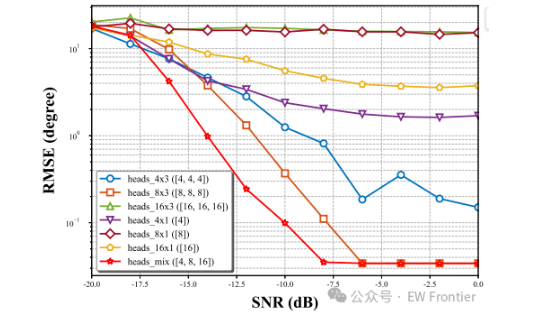

SNR(dB)	CMA-Former	DNN	CNN	DCT-ViT	HMC-ViT	MUSIC
-20	7.064	4.704	14.673	8.429	7.938	19.492
-16	0.475	1.313	3.230	0.559	0.619	12.667
-12	0.222	1.035	0.854	0.320	0.424	0.747
-10	0.194	0.848	0.621	0.263	0.435	0.333
0	0.191	0.491	0.587	0.203	0.467	0.191

模型规模与效率对比（V100）：

模型	参数量	FLOPs(G)	推理(ms)	训练显存(MB)
CMA-Former	1.57M	0.318	1.640	1637
CNN	28.19M	0.096	0.429	915
DCT-ViT	5.88M	0.388	0.777	661
HMC-ViT	2.41M	0.047	1.330	402
DNN	0.55M	0.001	0.298	318
MUSIC	-	-	0.719	-

关键结论：

低 SNR 区间（-16dB 以下）CMA-Former 优势显著，MUSIC 此时谱峰已完全失效（RMSE>12°）；
0dB 时 RMSE 0.191°，三源 CRB 约 0.089°，性能逼近理论下界；DNN 在 -16dB 后进入 0.85°~1.04° 平台期，拟合能力见顶；
HMC-ViT 在 -10dB 后停滞于 0.43°~0.47°，表征能力受限；DCT-ViT 表现最接近（-10dB 为 0.263°），验证了"序列化协方差特征 + Transformer"路线的有效性；
四源场景 -10dB 时 RMSE 0.46°，信源数增多对 CMA-Former 影响有限，而 MUSIC 在信源数超过 3 后基本失效；
效率：1.57M 参数（CNN 的 1/18）取得更优精度，单次推理 1.64ms，训练显存 1.6GB，消费级 GPU 完全可复现。

6. 踩坑总结

注意力头数：固定单头数效果差， $4,8,16$ 级联在低 SNR 下最优；
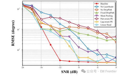
DropPath：建议随深度线性增加（scheduled），固定值导致深层训练震荡；
标签：hard 标签在网格边界震荡，高斯软标签（σ=2°）谱更平滑；
输入：全协方差矩阵（256 token）冗余且训练慢，上三角（120 token）更快更准；
位置编码：可学习位置编码在序列长度固定的任务中比正弦编码更灵活。

完整工程（数据生成、训练脚本、MUSIC/CNN/DNN/DCT-ViT/HMC-ViT 全套对比实验）见原文链接EWFrontier，回复「CMA-Former」获取。