线性二次调节器(Linear Quadratic Regulator,LQR)是针对线性系统的最优控制方法。LQR 方法标准的求解体系是在考虑到损耗尽可能小的情况下, 以尽量小的代价平衡其他状态分量。一般情况下,线性系统在LQR 控制方法中用状态空间方程描述,性能能指标函数由二次型函数描述。
LQR 方法存在以下优点:
- 最小能量消耗和最高路径跟踪精度。
- 求解时能够考虑多状态情况。
- 鲁棒性较强。
缺点:
- 控制效果和模型精确程度有很大相关性。
- 实时计算状态反馈矩阵和控制增益。
一、系统模型
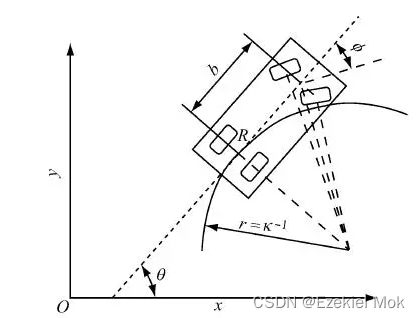
1.1 车辆模型
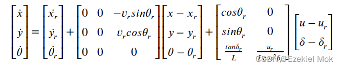
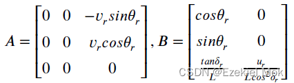
一般来说阿克曼移动机器人可以简化为自行车模型,是一个非线性时变系统,工程上一般通过在平衡点附近差分线性化转化为线性系统来分析和控制,具体就不推导了,我直接给出模型。
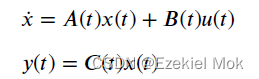
1.2 线性系统状态反馈控制示意图
状态反馈是线性能控线性系统镇定的一个有效方法,主要是通过极点配置方法寻找一组非正的闭环极点使得闭环系统大范围渐进稳定。
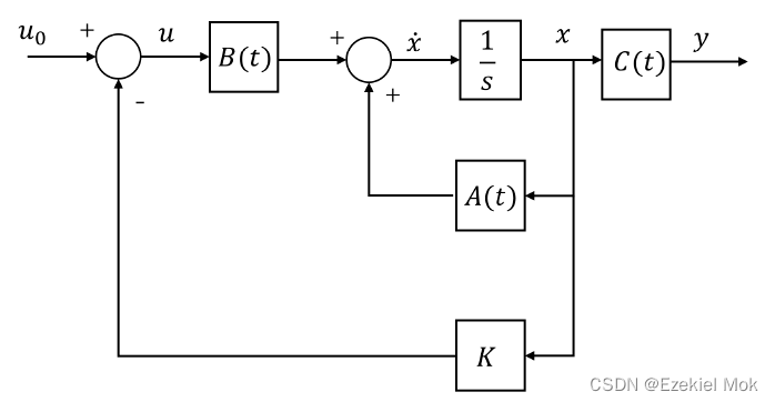
A,B,C分别代表系统矩阵、输入矩阵和输出矩阵,K是待设计的状态反馈增益。
二、控制器设计
2.1 代价函数泛函设计
最优控制里,代价函数一般设计为控制性能和控制代价的范数加权和,形式如下
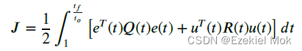
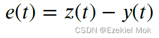
其中,期望和实际的误差系统定义为
2.2 最优状态反馈控制律推导
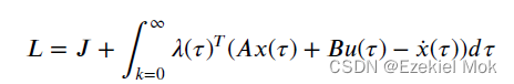
当想要状态与期望状态之间的误差越差越小,同时控制消耗更少的能量。求解极小值点时,新定义拉格朗日函数如下
在拉格朗日函数基础上对各个优化变量的一阶导为零 ,得
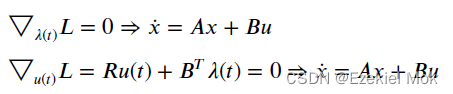
当时候,

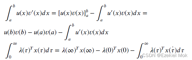
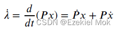
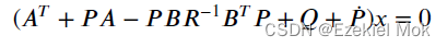
推导LQR控制律时候,设 ,求偏导后可得
由 得
得
由于状态量初始不为零,只能是
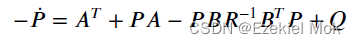
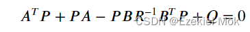
又由于当上述方程成立时候,收敛到了期望的范围 ,
为零,因此得到立卡提方程形式的矩阵微分方程
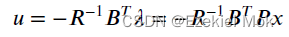
综上,通过迭代或者近似方法求解上述立卡提方程后,最优的控制律为
2.3 连续立卡提方程求解流程
三、具体实现代码
3.1 main函数
Matlab
close all
clear;
clc;
cx = [];
cy= [];
y0 = @(t_step) 10*sin(2 * t_step + 1);
x0_dot= @(t_step) 5 * 2 * cos(2 * t_step + 1);
x0 = @(t_step) -40*cos(t_step + 0.5);
for theta=0:pi/200:2*pi
    cx(end + 1) = x0(theta);
    cy(end + 1) = y0(theta);
end
refer_path_primary= [cx', cy'];
x = refer_path_primary(:, 1)';
y = refer_path_primary(:, 2)';
points = [x; y]';
ds = 0.1 ;%等距插值处理的间隔
distance = [0, cumsum(hypot(diff(x, 1), diff(y, 1)))]';
distance_specific = 0:ds:distance(end);
hypot(diff(x, 1), diff(y, 1));
diff(x, 1);
diff(y, 1);
s = 0:ds:distance(end);
refer_path= interp1(distance, points, distance_specific, 'spline');
figure(1)
% 绘制拟合曲线
plot(refer_path(:, 1), refer_path(:, 2),'b-',x, y,'r.');
hold on
refer_path_x = refer_path(:,1);  % x
refer_path_y = refer_path(:,2); % y
for i=1:length(refer_path)
    if i==1
         dx = refer_path(i + 1, 1) - refer_path(i, 1);
         dy = refer_path(i + 1, 2) - refer_path(i, 2);
         ddx = refer_path(3, 1) + refer_path(1, 1) - 2 * refer_path(2, 1);
         ddy = refer_path(3, 2) + refer_path(1, 2) - 2 * refer_path(2, 2);
    elseif  i==length(refer_path)
         dx = refer_path(i, 1) - refer_path(i - 1, 1);
         dy = refer_path(i, 2) - refer_path(i - 1, 2);
         ddx = refer_path(i, 1) + refer_path(i - 2, 1) - 2 * refer_path(i - 1, 1);
         ddy = refer_path(i, 2) + refer_path(i - 2, 2) - 2 * refer_path(i - 1, 2);
    else
          dx = refer_path(i + 1, 1) - refer_path(i, 1);
          dy = refer_path(i + 1, 2) - refer_path(i, 2);
          ddx = refer_path(i + 1, 1) + refer_path(i - 1, 1) - 2 * refer_path(i, 1);
          ddy = refer_path(i + 1, 2) + refer_path(i - 1, 2) - 2 * refer_path(i, 2);
    end
    refer_path(i,3)=atan2(dy, dx);%yaw
    refer_path(i,4)=(ddy * dx - ddx * dy) / ((dx ^ 2 + dy ^ 2) ^ (3 / 2));
end
figure(2)
plot(refer_path(:, 3),'b-');
figure(3)
plot(refer_path(:, 4),'b-')
%
%%目标及初始状态
L=2;%车辆轴距
v=2;%初始速度
dt=0.05;%时间间隔
goal=refer_path(end,1:2);
x_0=refer_path_x(1);
y_0=refer_path_y(1);
psi_0 = refer_path(1, 3);
% %运动学模型
ugv = KinematicModel(x_0, y_0, psi_0, v, dt, L);
Q = eye(3) * 3.0;
R = eye(2) * 2.0;
robot_state = zeros(4, 1);
step_points = length(refer_path(:, 1));
for i=1:1:step_points
    robot_state(1)=ugv.x;
    robot_state(2)=ugv.y;
    robot_state(3)=ugv.psi;
    robot_state(4)=ugv.v;
    [e, k, ref_yaw, min_idx] = calc_track_error(robot_state(1), robot_state(2), refer_path);
    ref_delta = atan2(L * k, 1);
    [A, B] = state_space( robot_state(4), ref_delta, ref_yaw, dt, L);
    delta = lqr(robot_state, refer_path, min_idx, A, B, Q, R);
    delta = delta + ref_delta;
    [ugv.x, ugv.y, ugv.psi, ugv.v] = update(0, delta, dt, L, robot_state(1), robot_state(2),robot_state(3), robot_state(4));
    ugv.record_x(end + 1 ) = ugv.x;
    ugv.record_y(end + 1 ) = ugv.y;
    ugv.record_psi(end + 1 ) = ugv.psi;
     ugv.record_phy(end + 1 ) = ref_delta;
end
figure(4)
% 绘制拟合曲线
%  scr_size = get(0,'screensize');
% set(gcf,'outerposition', [1 1 scr_size(4) scr_size(4)]);
plot(ugv.record_x , ugv.record_y, Color='m',LineStyle='--',LineWidth=2);
axis([-40,40,-40,40])
grid on
hold on
% 绘制车辆曲线
axis equal
for ii = 1:1:length(ugv.record_x)

        h =  PlotCarbox(ugv.record_x(ii), ugv.record_y(ii), ugv.record_psi(ii), 'Color', 'r',LineWidth=2);
        h1 = plot(ugv.record_x(1:ii), ugv.record_y(1:ii),'Color', 'b');
        th1 = text(ugv.record_x(ii), ugv.record_y(ii)+10, ['#car', num2str(1)], 'Color', 'm');
        set(th1, {'HorizontalAlignment'},{'center'});
        h2 = PlotCarWheels(ugv.record_x(ii), ugv.record_y(ii), ugv.record_psi(ii),ugv.record_phy(ii),'k',LineWidth=2);
        h3 = plot(ugv.record_x(1:ii) , ugv.record_y(1:ii), Color='b',LineStyle='-',LineWidth=4);
        drawnow
        delete(h); delete(h1);delete(th1);delete(h3);
        for jj = 1:1:size(h2)
            delete(h2{jj});
        end
end
%
function [P] =  cal_Ricatti(A, B, Q, R)
 Qf = Q;
 P = Qf;
  iter_max = 100;
  Eps = 1e-4;
 for step = 1:1:iter_max
     P_bar = Q + A' * P * A - A' * P * B * pinv(R + B' * P *B) * B' * P * A;
     criteria = max(abs(P_bar - P));
     if  criteria < Eps
         break;
     end
     P = P_bar;
 end

end
%%LQR控制器
function[u_star]=lqr(robot_state, refer_path, s0, A, B, Q, R)
    x = robot_state(1:3) - refer_path(s0,1:3)';
    P =  cal_Ricatti(A, B, Q, R);
    K= -pinv(R + B' * P * B) * B' * P * A;
    u = K * x;%状态反馈
    u_star = u(2);
end

function [e, k, yaw, min_idx]=calc_track_error(x, y, refer_path)
    p_num = length(refer_path);
    d_x = zeros(p_num, 1);
    d_y = zeros(p_num, 1);
    d = zeros(p_num, 1);
    for i=1:1:p_num
        d_x(i) = refer_path(i, 1) - x;
        d_y(i) = refer_path(i, 2) - y;
    end
    for i=1:1:p_num
        d(i) = sqrt(d_x(i) ^2 + d_y(i) ^ 2) ;
    end
    [~, min_idx] = min(d);
    yaw = refer_path(min_idx, 3);
    k = refer_path(min_idx, 4);
    angle= normalize_angle(yaw - atan2(d_y(min_idx), d_x(min_idx)));
    e = d(min_idx);
    if angle < 0
        e = e*(-1);
    end
end
%%将角度取值范围限定为[-pi,pi]
function [angle]=normalize_angle(angle)
    while angle > pi
        angle = angle - 2*pi;
    end
    while angle < pi
        angle = angle + 2*pi;
    end
end
function [x_next, y_next, psi_next, v_next] = update(a, delta_f, dt, L, x, y, psi, v)
     x_next = x + v * cos(psi) * dt;
     y_next = y + v * sin(psi) * dt;
     psi_next = psi + v / L * tan(delta_f) * dt;
     v_next = v + a * dt;
end
function [A, B]=state_space(v, ref_delta, ref_yaw, dt, L)
    A=[ 1.0, 0.0,  -v * dt * sin(ref_yaw);
           0.0, 1.0,   v *  dt * cos(ref_yaw);
           0.0, 0.0,   1.0  ];
    B =[ dt * cos(ref_yaw), 0;
           dt * sin(ref_yaw), 0;
           dt * tan(ref_delta) / L, v * dt / (L * cos(ref_delta) * cos(ref_delta))];
end
function h = PlotCarbox(x, y, theta, varargin)
Params = GetVehicleParams();

carbox = [-Params.Lr -Params.Lb/2; Params.Lw+Params.Lf -Params.Lb/2; Params.Lw+Params.Lf Params.Lb/2; -Params.Lr Params.Lb/2];
carbox = [carbox; carbox(1, :)];

transformed_carbox = [carbox ones(5, 1)] * GetTransformMatrix(x, y, theta)';
h = plot(transformed_carbox(:, 1), transformed_carbox(:, 2), varargin{:});

end
function hs = PlotCarWheels(x, y, theta, phy, varargin)
Params = GetVehicleParams();

wheel_box = [-Params.wheel_radius -Params.wheel_width / 2;
    +Params.wheel_radius -Params.wheel_width / 2;
    +Params.wheel_radius +Params.wheel_width / 2;
    -Params.wheel_radius +Params.wheel_width / 2];

front_x = x + Params.Lw * cos(theta);
front_y = y + Params.Lw * sin(theta);
track_width_2 = (Params.Lb - Params.wheel_width / 2) / 2;

boxes = {
    TransformBox(wheel_box, x - track_width_2 * sin(theta), y + track_width_2 * cos(theta), theta);
    TransformBox(wheel_box, x + track_width_2 * sin(theta), y - track_width_2 * cos(theta), theta);
    TransformBox(wheel_box, front_x - track_width_2 * sin(theta), front_y + track_width_2 * cos(theta), theta+phy);
    TransformBox(wheel_box, front_x + track_width_2 * sin(theta), front_y - track_width_2 * cos(theta), theta+phy);
};

hs = cell(4, 1);
for ii = 1:4
    hs{ii} = fill(boxes{ii}(:, 1), boxes{ii}(:, 2), varargin{:});
end

end

function transformed = TransformBox(box, x, y, theta)
transformed = [box; box(1, :)];
transformed = [transformed ones(5, 1)] * GetTransformMatrix(x, y, theta)';
transformed = transformed(:, 1:2);
end
function mat = GetTransformMatrix(x, y, theta)
mat = [ ...
    cos(theta) -sin(theta), x; ...
    sin(theta) cos(theta), y; ...
    0 0 1];
end
3.2 运动学结构体:
Matlab
classdef  KinematicModel<handle
    properties
        x;
        y;
        psi;
        v;
        dt;
        L;
        record_x;
        record_y;
        record_psi;
        record_phy;
    end
    methods
        function self=KinematicModel(x, y, psi, v, dt, L)
            self.x=x;
            self.y=y;
            self.psi=psi;
            self.v = v;
            self.L = L;
            % 实现是离散的模型
            self.dt = dt;
            self.record_x = [];
            self.record_y= [];
            self.record_psi= [];
            self.record_phy= [];
        end
end
end
四、仿真参数和效果
4.1 参数配置
Matlab
%期望轨迹
y0 = @(t_step) 10*sin(2 * t_step + 1);
x0_dot= @(t_step) 5 * 2 * cos(2 * t_step + 1);
L=2;%车辆轴距
v=2;%初始速度
dt=0.05;%时间间隔
Q = eye(3) * 3.0;
R = eye(2) * 2.0;
robot_state = zeros(4, 1);
VehicleParams.Lw = 2.8 * 2; % wheel base
VehicleParams.Lf = 0.96 * 2; % front hang
VehicleParams.Lr = 0.929 * 2; % rear hang
VehicleParams.Lb = 1.942 * 2; % width
VehicleParams.Ll = VehicleParams.Lw + VehicleParams.Lf + VehicleParams.Lr; % length
VehicleParams.f2x = 1/4 * (3*VehicleParams.Lw + 3*VehicleParams.Lf - VehicleParams.Lr);
VehicleParams.r2x = 1/4 * (VehicleParams.Lw + VehicleParams.Lf - 3*VehicleParams.Lr);
VehicleParams.radius = 1/2 * sqrt((VehicleParams.Lw + VehicleParams.Lf + VehicleParams.Lr) ^ 2 / 4 + VehicleParams.Lb ^ 2);
VehicleParams.a_max = 0.5;
VehicleParams.v_max = 2.5;
VehicleParams.phi_max = 0.7;
VehicleParams.omega_max = 0.5;
% for wheel visualization
VehicleParams.wheel_radius = 0.32*2;
VehicleParams.wheel_width = 0.22*2;
iter_max = 100;
Eps = 1e-4;
4.1 仿真效果