文章目录
-
-
- [1.Simple linear regression](#1.Simple linear regression)
- [2.Simple linear correlation](#2.Simple linear correlation)
-
方差分析
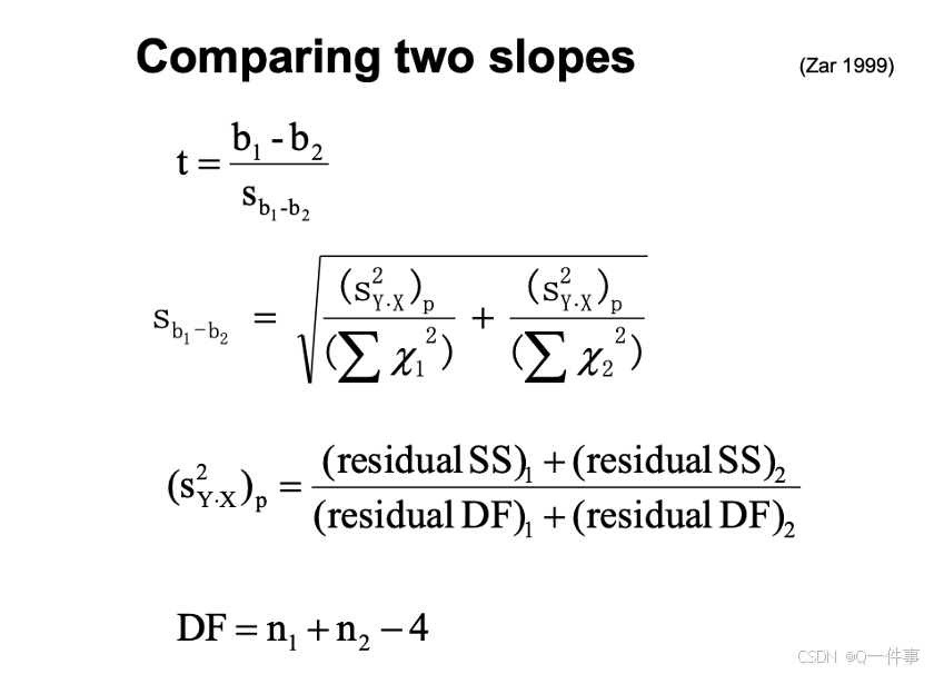
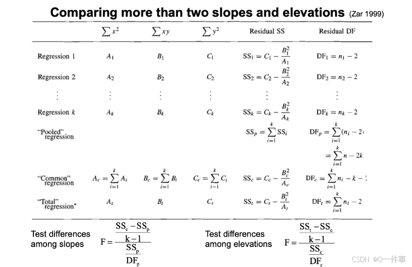
组间差异和
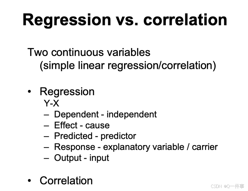
分类变量解释连续变量的情况用回归和相关。
线性回归是因果分析,相关性没有因果分析。
1.Simple linear regression
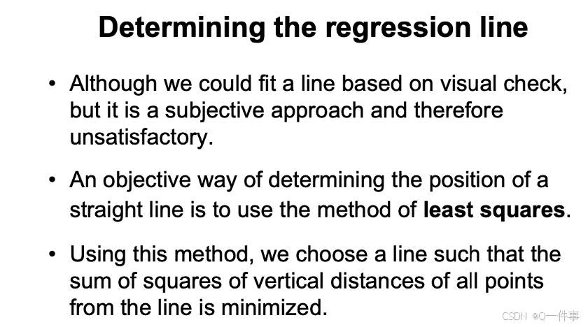
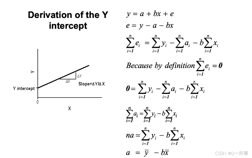
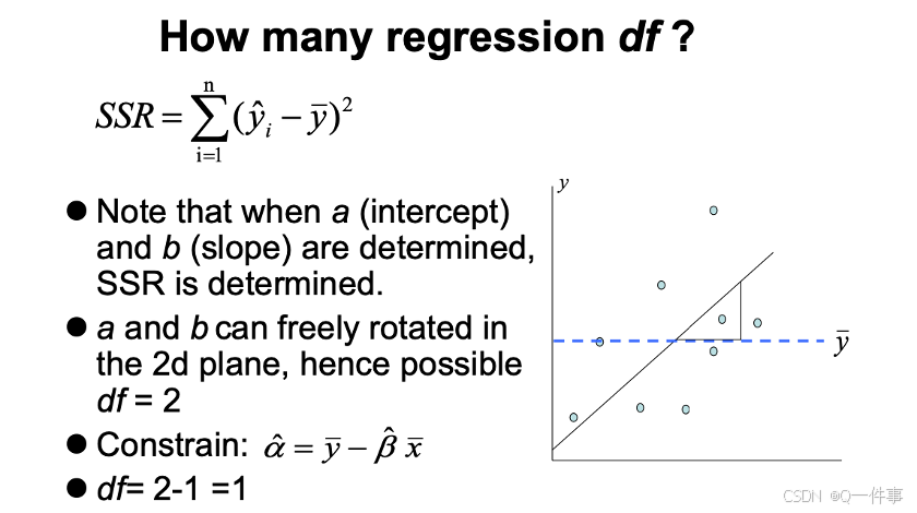
让残差最小。
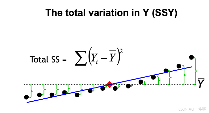
是斜率b, x的平方的加和是总变异。
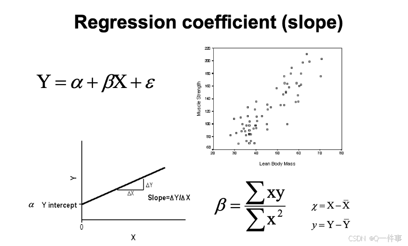
回归分析也是线性模型,方差具有可加性。
每个都可以计算。
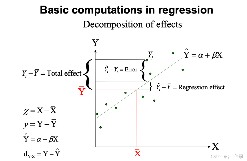
y的总变异。
{r}
plot(trees$Girth, trees$Height)
abline(lm(trees$Height~trees$Girth))
X = trees$Girth
Y = trees$Height

# The famous five sums
sum(X)
sum(X^2)
sum(Y)
sum(Y^2)
sum(X*Y)


sum(X);sum(X^2);sum(Y);sum(Y^2);sum(X*Y)
# matrix multiplication
XY <- cbind(1,X,Y)
t(XY) %*% XY
式子是相等的。
{r}
# Sums of squares and sums of products
SSX = sum((X-mean(X))^2); SSX
SSY = sum((Y-mean(Y))^2); SSY
SSXY = sum((Y-mean(Y))*(X-mean(X))); SSXY

# 后面的是前面的
# The alternative way using the 5 sums
SSX = sum(X^2)-sum(X)^2/length(X); SSX
SSY = sum(Y^2)-sum(Y)^2/length(Y); SSY
SSXY = sum(X*Y)-sum(X)*sum(Y)/length(X); SSXY
{r}
# Model (Y=a+bX) coefficients
b = SSXY/SSX; b
a = mean(Y)-b*mean(X); a
lm(Y~X)
证明:生成这条直线是过均值点的。
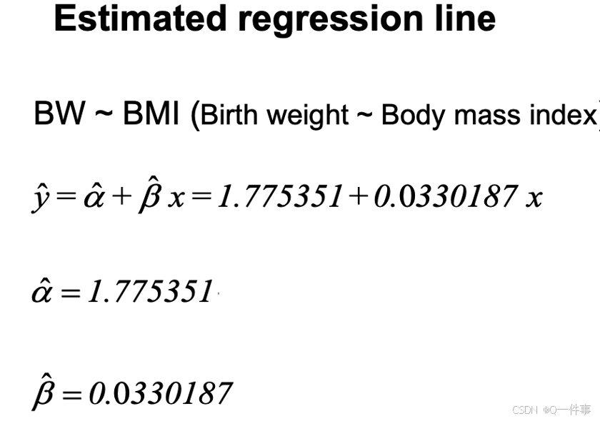
连续变量需要减去一个变量。
{r}
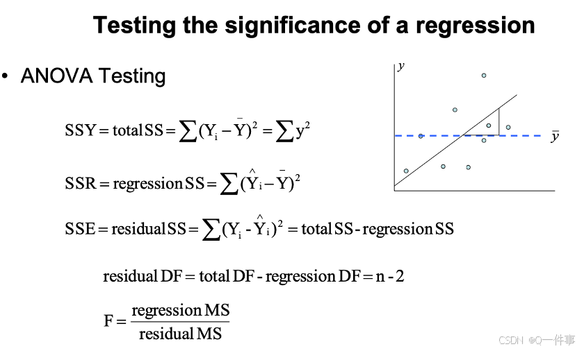
# Analysis of variance in regression
anova(lm(Y~X)) # data: trees
qf(0.95,1,29) # 4.18
1-pf(10.707,1,29)
{r}
# Unreliability estimates for the parameters
summary(lm(Y~X))
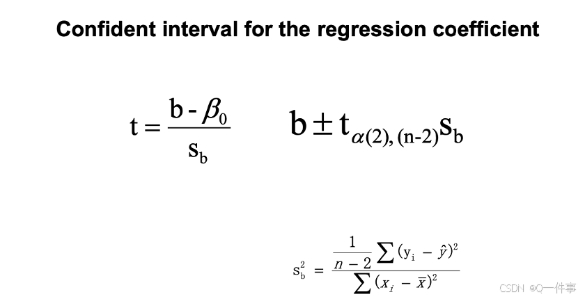
confint(lm(Y~X))斜率的标准error表明
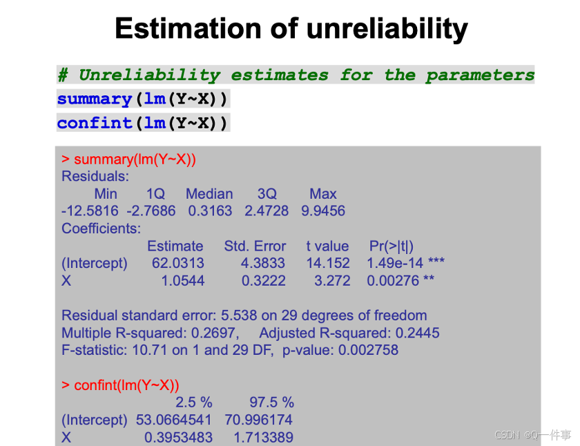
模型中x解释的变异。使得残差最小,然后就是R方最大。
{r}
# Degree of scatter
SSY = deviance(lm(Y~1)); SSY # SSY
SSE = deviance(lm(Y~X)); SSE # SSE
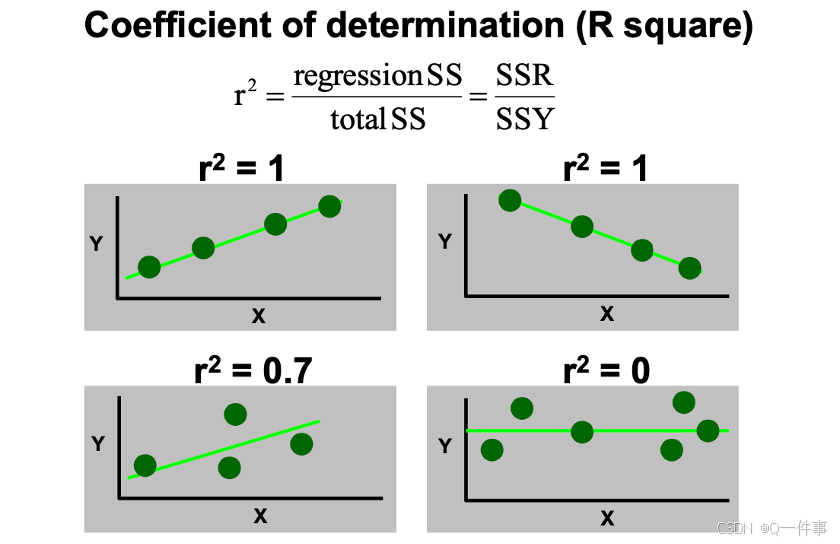
rsq = (SSY-SSE)/SSY; rsq # R square
summary(lm(Y~X))[[8]]下面的代码是R方和调整过的R方。事实上,当涉及到多变量的时候,会用调整后的R方。
{r}
summary(lm(Volume~Girth, trees))$r.squared

# 当涉及到多个变量时候,会进行矫正
summary(lm(Volume~Girth, trees))$adj.r.squared
n是记录的行数,数据量大的话不支持多个变量。
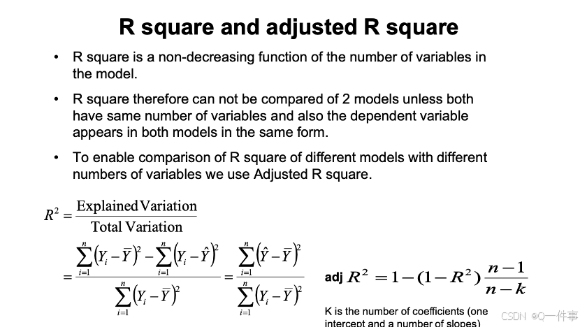
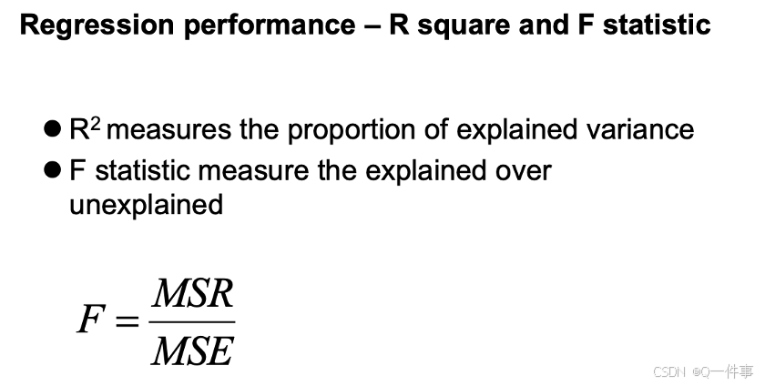
各个名词的区别。R方是用来解释能解释的变异。F 统计量衡量已解释的数占未解释数的比例
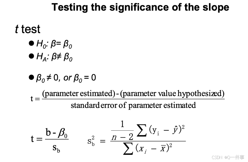
这里计算的t值和后文有较大的关系。
{r}
summary(lm(Y~X))[[4]][4] # The standard error of the slope
summary(lm(Y~X))[[4]]
中间是最准的。样本量越大,预测越准。
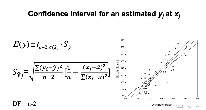
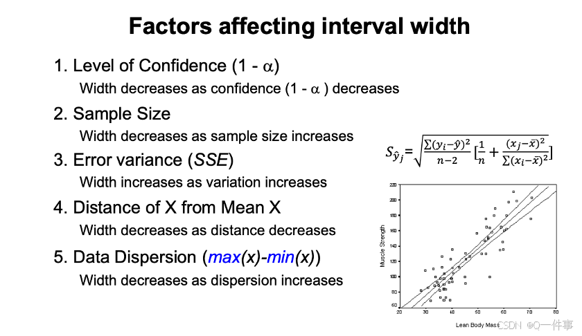
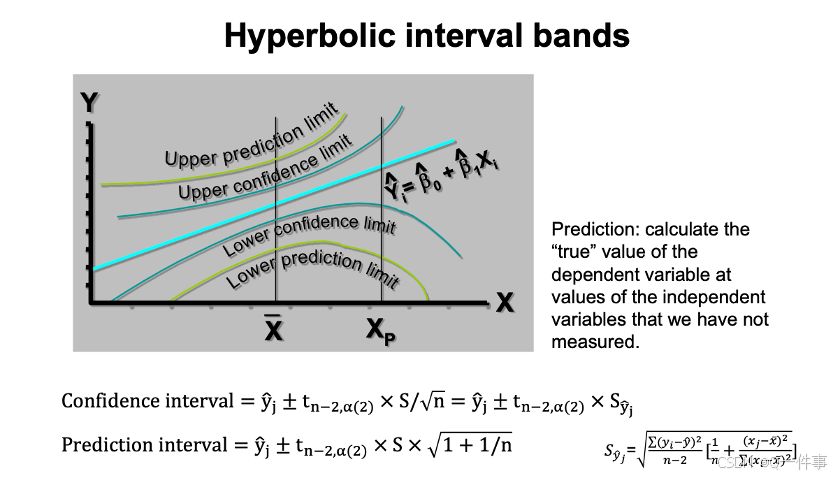
这个是实验设计。
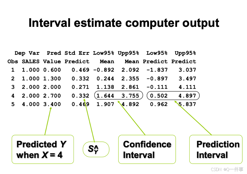
预测空间在外面,置信空间在里面。
{r}
# Prediction using the fitted model
model <- lm(Y~X)
predict(model, list(X = c(14,15,16)))
{r}
ci.lines<-function(model){
xm <- mean(model[[12]][,2])
n <- length(model[[12]][[2]])
ssx<- sum(model[[12]][2]^2)- sum(model[[12]][2])^2/n
s.t<- qt(0.975,(n-2))
xv <- seq(min(model[[12]][2]),max(model[[12]][2]),
(max(model[[12]][2])-min(model[[12]][2]))/100)
yv <- coef(model)[1]+coef(model)[2]*xv
se <- sqrt(summary(model)[[6]]^2*(1/n+(xv-xm)^2/ssx))
ci <- s.t * se
uyv<- yv + ci
lyv<- yv - ci
lines(xv, uyv, lty=2)
lines(xv, lyv, lty=2)
}
plot(X, Y, pch = 16)
abline(model)
ci.lines(model)
# Another method
X = trees$Girth; Y = trees$Height
model <- lm(Y~X)
plot(X, Y, pch = 16, ylim=c(60,95))
xv <- seq(8,22,1)
y.c <- predict(model,list(X=xv),int="c") # "c": 95% CI
y.p <- predict(model,list(X=xv),int="p") # "p": prediction
matlines(xv, y.c, lty=c(1,2,2), lwd=2, col="black")
matlines(xv, y.p, lty=c(1,2,2), lwd=1, col=c("black","grey","grey"))
x的总变异,y的总变异。
{r}
x1 <- rep( 0:1, each=500 ); x2 <- rep( 0:1, each=250, length=1000 )
y <- 10 + 5*x1 + 10*x2 - 3*x1*x2 + rnorm(1000,0,2) #values
fit1 <- lm( y ~ x1*x2 )
newdat <- expand.grid( x1=0:1, x2=0:1 )
pred.lm.ci <- predict(fit1, newdat, interval='confidence')
pred.lm.pi <- predict(fit1, newdat, interval='prediction')
pred.lm.ci; pred.lm.pi
# function for plotting error bars from http://monkeysuncle.stanford.edu/?p=485
error.bar <- function(x, y, upper, lower=upper, length=0.1,...){
if(length(x) != length(y) | length(y) !=length(lower) | length(lower) != length(upper))
stop("vectors must be same length")
arrows(x,y+upper, x, y-lower, angle=90, code=3, length=length, ...)}
barx <- barplot(pred.lm.ci[,1], names.arg=1:4, col="blue", axis.lty=1, ylim=c(0,28),
xlab="Levels", ylab="Values")
# Error bar for confidence interval
error.bar(barx, pred.lm.ci[,1], pred.lm.ci[,2]-pred.lm.ci[,1],pred.lm.ci[,1]-pred.lm.ci[,3])
# Error bar for prediction interval
error.bar(barx, pred.lm.pi[,1], pred.lm.pi[,2]-pred.lm.pi[,1],pred.lm.pi[,1]-pred.lm.pi[,3],col='red')
{r}
# Model checking
par(mfrow=c(2,2)); plot(model)
(1)影响因子
影响因素是不一样的。
x和观测值变化一点点,对模型影响的程度。
回归线最边上的点的变化对影响是非常大的。
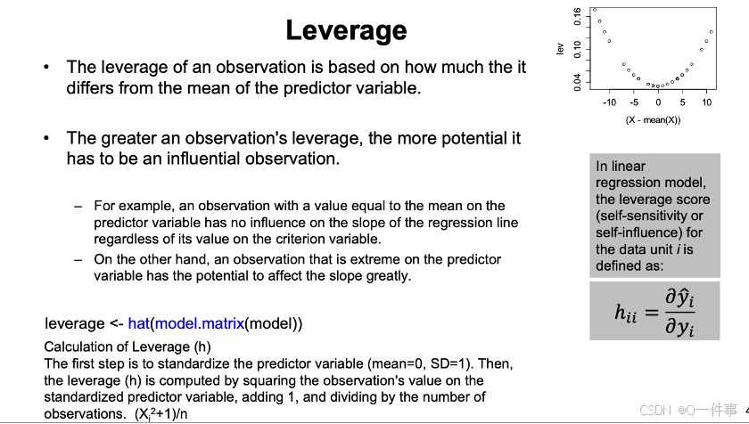
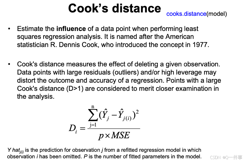
丢点这个点,对预测值的影响的大小。是对整体的影响。
{r}
# 计算贡献后,计算其斜率
# Model update (remove one outlier)
model2 <- update(model,subset=(X != 15))
summary(model2)
# Slope
coef(model2)[2] # 1.054369
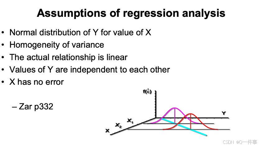
model2$coefficients[2] # 1.054369(2)线性回归的假定
线性回归不需要x和y分别正态,是要对应x上y上正态分布
方差齐性
线性关系
x没有错误
s代表啥意思呢?这个部分我还是没弄太明白。
{r}
reg.tree <- lm(Volume~Height, data=trees)
reg.tree
{r}
summary(reg.tree)
{r}
par(mfrow=c(2,2))
plot(lm(Volume~Height, data=trees))
检查几种情况
{r}
library(car)
fit = lm(Girth ~ Height, data = trees)
# Computes residual autocorrelations and generalized Durbin-Watson statistics
# and their bootstrapped p-values
durbinWatsonTest(fit) # check independence
# P < 0.05, autocorrelation exists.
# component + residual plots (also called partial-residual plots) for linear
# and generalized linear models
crPlots(fit) # check linearity
# the red line (regression) and green line (residual) match well, the linearity is good.
# Score Test for Non-Constant Error Variance
ncvTest(fit) #检查方差齐性的方法
# p = 0.15, error variance is homogeneous
回归中看p值中,看斜率的p值。截距p值过大,则可以将其视为0.
2.Simple linear correlation
{r}
# correlation coefficient and p value
cor(X, Y, use = 'pairwise.complete.obs')
cor.test(X, Y, alternative = c("two.sided"), method = c("pearson"))$p.value


# correlation coefficient
r = SSXY/(SSX*SSY)^.5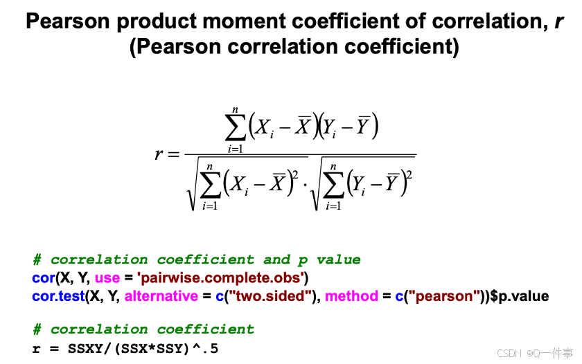
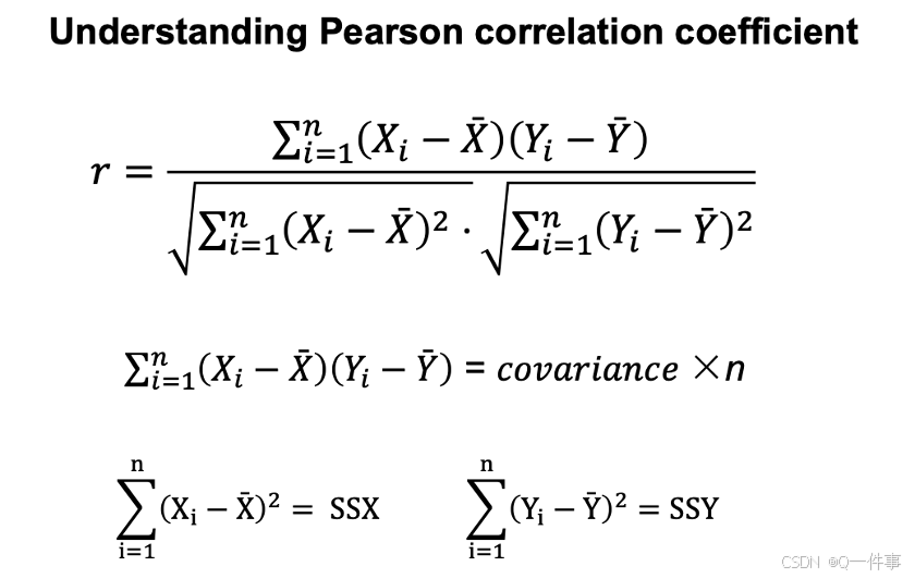
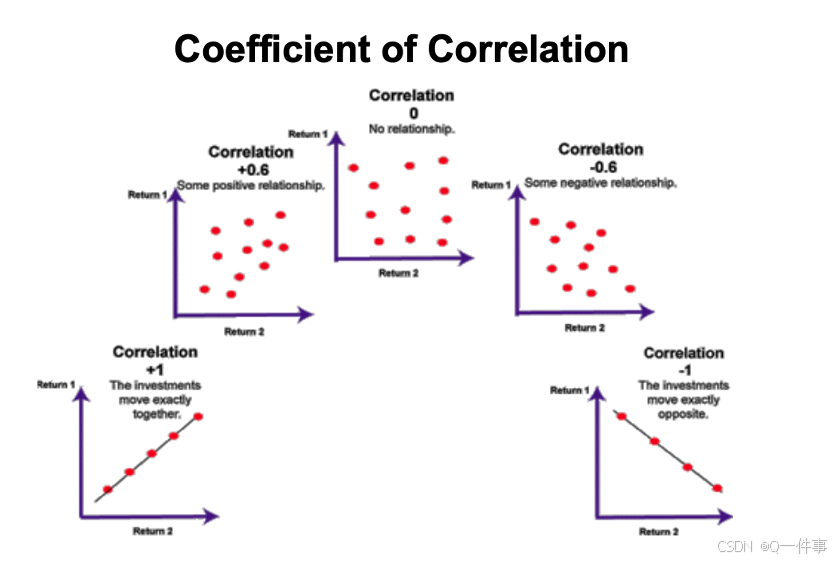
对相关系数的解释
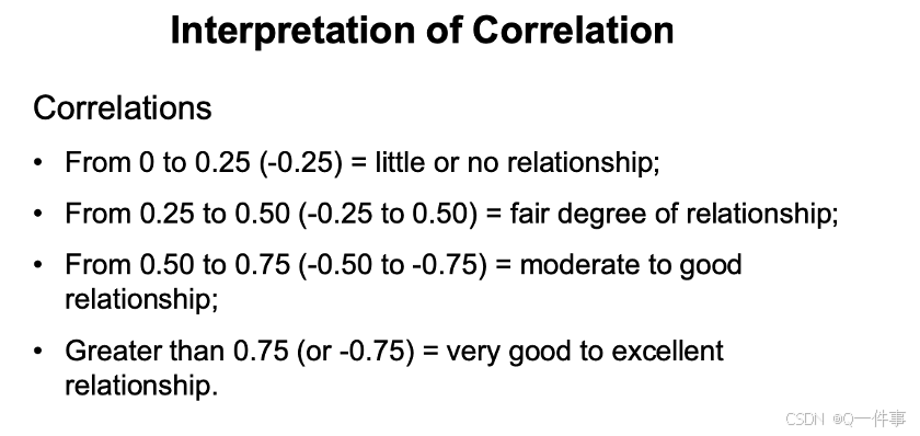
(1)相关性的解释
对相关性的解释
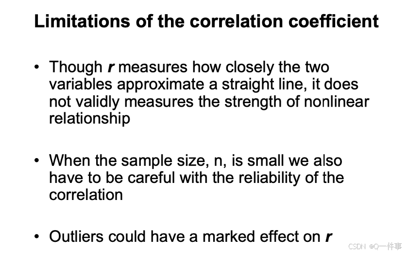
相关系数的误差可以这样看出来。
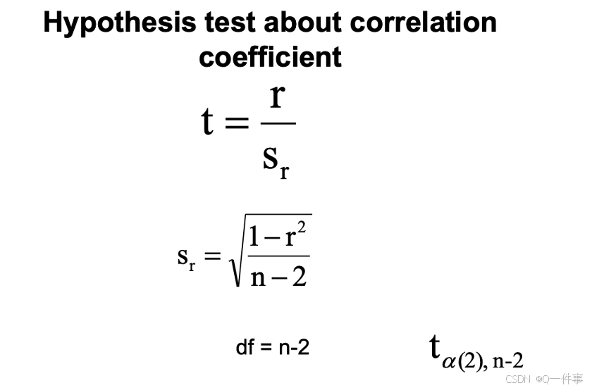
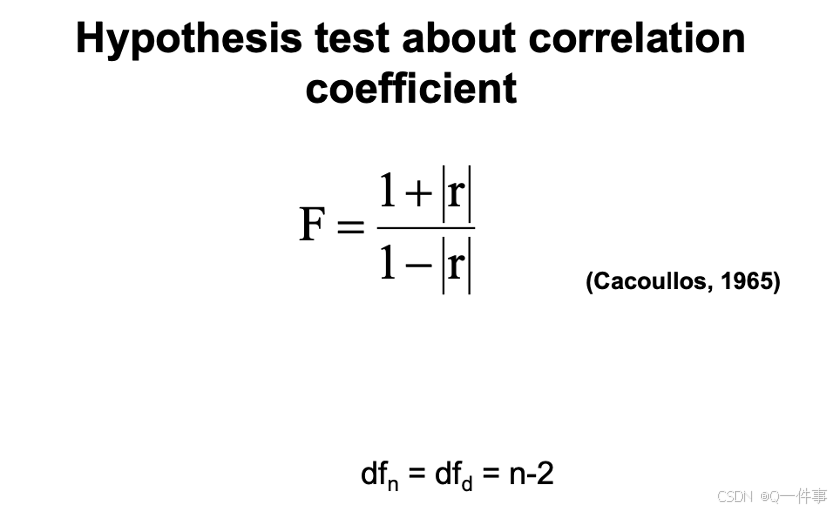
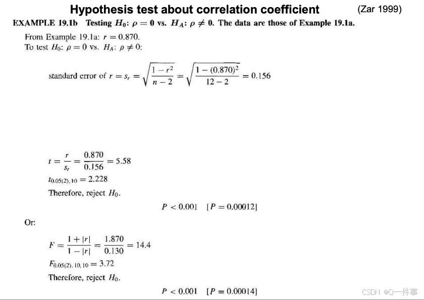
认为这种可能是偶然的情况。即事实上也需要对其进行t检验。
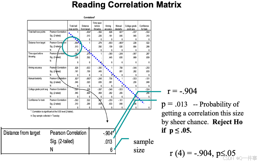
相关性的假设检验

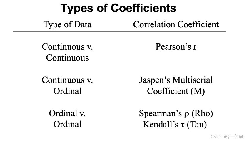
(2)不同的相关性
bash
head(mtcars)
plot(mtcars$wt, mtcars$hp)
# Pearson correlation coefficient
cor(mtcars$wt, mtcars$hp) # 0.66
wt.rank = rank(mtcars$wt)
hp.rank = rank(mtcars$hp)
# Spearman correlation coefficient
cor(wt.rank, hp.rank) # 0.77
X = seq(0.5* pi, 1.5*pi, length=100)
Y = 1 - sin(X)
plot(Y, X)
cor(X, Y) # 0.99
cor(rank(X),rank(Y)) # 1
Hmisc这个可以做各种各样的相关系数
library(Hmisc)

head(mtcars)
rcorr(as.matrix(mtcars), type="pearson")
rcorr(as.matrix())
样本量和相关系数决定量p值
连续变量对连续变量的关系