用 Python 从零开始创建神经网络（十五）：Dropout

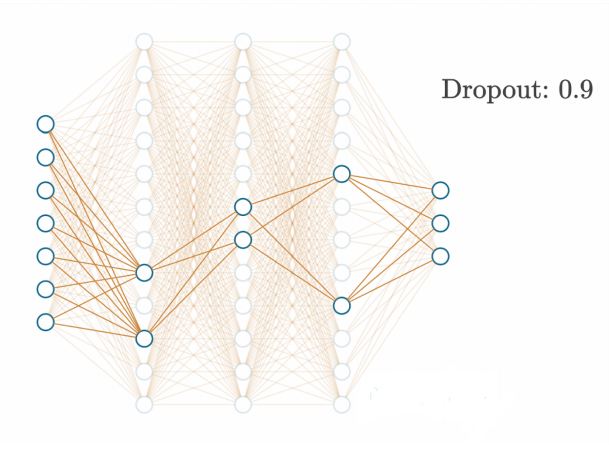
Dropout

• 引言
• [1. Forward Pass](#1. Forward Pass)
• [2. Backward Pass](#2. Backward Pass)
• [3. 代码](#3. 代码)
• 到目前为止的全部代码：

引言

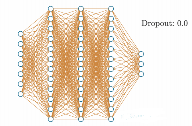
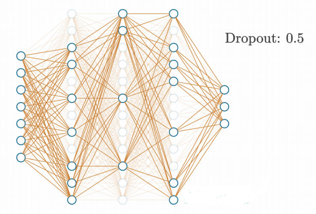
另一种用于神经网络正则化的选项是添加一个dropout层。这种类型的层会禁用一些神经元，而让其他神经元保持不变。其理念与正则化类似，是为了防止神经网络对任何一个神经元的依赖过高，或在某个特定实例中完全依赖某个神经元（这在模型过拟合训练数据时很常见）。dropout还能帮助解决另一个问题，即共适应现象（co-adoption）。共适应是指神经元依赖其他神经元的输出值，而不能独立学习底层函数。通过让更多的神经元共同工作，dropout还能应对训练数据中的噪声和其他扰动，这使得模型能够学习更复杂的函数。

Dropout函数通过在每次前向传播中随机禁用一定比例的神经元来工作，这迫使网络必须学会在仅剩一部分随机选中的神经元的情况下依然进行准确的预测。Dropout强迫模型使用更多的神经元来完成相同的任务，从而提高学习描述数据底层函数的能力。例如，如果在当前步骤禁用一半的神经元，在下一步骤禁用另一半神经元，我们就强迫更多的神经元学习数据，因为只有部分神经元能够"看到"数据并在某次传播中得到更新。这种交替使用一半神经元的方式仅仅是一个例子，实际上我们会使用一个超参数来通知dropout层随机禁用的神经元数量。

此外，由于活跃的神经元是动态变化的，dropout有助于防止过拟合，因为模型不能依赖特定神经元来记住某些样本。同样需要提到的是，dropout层实际上并没有真正禁用神经元，而是将它们的输出置为零。换句话说，dropout既不会减少使用的神经元数量，也不会让训练过程在禁用一半神经元时快一倍。

1. Forward Pass

在代码中，我们将使用一个过滤器"关闭"神经元，这个过滤器是一个与层输出形状相同的数组，其中填充了从伯努利分布中抽取的数字。伯努利分布是一种二元（或离散）概率分布，其中我们可以以概率 p p p获得值1，以概率 q q q获得值0。让我们从这个分布中取一个随机值 r i r_i ri，则有：

这意味着该值为1的概率是 p p p，而其为0的概率是 q = 1 − p q = 1 - p q=1−p，因此：

这意味着给定的 r i r_i ri是来自伯努利分布的值，其取值为1的概率是 p p p。如果 r i r_i ri是该分布中的一个单独值，则可以从该分布中抽取一个值，并将其重新整形以匹配层输出的形状，用作这些输出的掩码。

我们得到一个数组，其中以概率 p p p填充值为1，其余为0的值。然后我们将该过滤器应用于希望添加Dropout的层的输出。

代码引用：https://nnfs.io/def

在代码中，Dropout层有一个超参数。这是一个值，用于指定在该层中需要禁用的神经元的百分比。例如，如果选择了0.10作为Dropout参数，则每次前向传播中将随机禁用10%的神经元。在使用NumPy之前，我们将通过一个纯Python的示例来演示这一点：

import random

dropout_rate = 0.5
# Example output containing 10 values
example_output = [0.27, -1.03, 0.67, 0.99, 0.05, -0.37, -2.01, 1.13, -0.07, 0.73]

# Repeat as long as necessary
while True:
    
    # Randomly choose index and set value to 0
    index = random.randint(0, len(example_output) - 1)
    example_output[index] = 0
    
    # We might set an index that already is zeroed
    # There are different ways of overcoming this problem,
    # for simplicity we count values that are exactly 0
    # while it's extremely rare in real model that weights
    # are exactly 0, this is not the best method for sure
    dropped_out = 0
    for value in example_output:
        if value == 0:
            dropped_out += 1
            
    # If required number of outputs is zeroed - leave the loop
    if dropped_out / len(example_output) >= dropout_rate:
        break
print(example_output)

>>>
[0, -1.03, 0.67, 0.99, 0, -0.37, 0, 0, 0, 0.73]

代码相对基础，但其思想是随机将神经元的输出置为0，直到禁用达到目标百分比的神经元。如果我们将伯努利分布视为二项分布的一个特殊情况（ n = 1 n=1 n=1），并查看NumPy中可用的方法列表，会发现使用numpy.random.binomial可以更简洁地实现这一目标。二项分布与伯努利分布的唯一区别是增加了一个参数 n n n，即并发实验的次数（而不仅仅是一次实验），并返回这些 n n n次实验中的成功次数。

np.random.binomial()通过接受前面讨论过的参数 n n n（实验次数）和 p p p（实验结果为1的概率）以及一个额外的参数size来工作：np.random.binomial(n, p, size)。

这个函数本质上可以被视为一次掷硬币实验，其中结果将是0或1。参数 n n n表示你想要掷硬币的次数， p p p是掷硬币结果为1的概率。总体结果是所有掷硬币结果的总和。参数size表示要运行多少次这样的"实验"，返回的是一个总体结果的列表。例如：

import random
import numpy as np

binomial_results = np.random.binomial(2, 0.5, size=10)
print(binomial_results)

这将生成一个大小为10的数组，其中每个元素是两次掷硬币结果的总和，掷硬币结果为1的概率为0.5或50%。生成的数组如下：

>>>
[0 2 1 1 2 1 0 1 1 1]

我们可以使用上述方法创建一个Dropout层。这里的目标是创建一个滤波器，其中表示目标Dropout百分比的部分为0，其余部分为1。例如，假设我们有一个包含5个神经元的层，在其后添加一个Dropout层，并希望实现20%的Dropout率。那么，理想状态下一个Dropout层的示例如下：

[1, 0, 1, 1, 1]

如你所见，这个列表的五分之一是0。这就是我们将应用于全连接层输出的滤波器的一个示例。如果将神经网络层的输出与这个滤波器相乘，就会有效地禁用与0对应的索引处的神经元。

我们可以通过以下方式使用np.random.binomial()来模拟这一过程：

dropout_rate = 0.20
np.random.binomial(1, 1-dropout_rate, size=5)

import random
import numpy as np

dropout_rate = 0.20
binomial_results = np.random.binomial(1, 1-dropout_rate, size=5)
print(binomial_results)

>>>
[1 0 1 1 1]

这是基于概率的，因此有时生成的数组可能不会像上面的示例那样。有可能没有神经元被置零，或者所有神经元都被置零。但总体上，这些随机抽样会趋向于我们期望的概率值。此外，上述示例使用了一个非常小的层（5个神经元）。在实际规模的层中，您会发现概率更一致地匹配您设定的目标值。

假设一个神经网络层的输出是：

example_output = np.array([0.27, -1.03, 0.67, 0.99, 0.05, -0.37, -2.01, 1.13, -0.07, 0.73])

接下来，假设我们的目标Dropout率为 0.3，即 30%。我们应用Dropout层：

import random
import numpy as np

dropout_rate = 0.3
example_output = np.array([0.27, -1.03, 0.67, 0.99, 0.05, -0.37, -2.01, 1.13, -0.07, 0.73])
example_output *= np.random.binomial(1, 1-dropout_rate, example_output.shape)

print(example_output)

>>>
[ 0.27 -1.03  0.67  0.99  0.05 -0.37 -2.01  1.13 -0.    0.73]

请注意，我们的dropout率是我们计划禁用的神经元比例（ q q q）。有时，dropout的实现会包含一个rate参数，它表示我们计划保留的神经元比例（ p p p）。在本文写作时，深度学习框架TensorFlow和Keras中的dropout参数表示您计划禁用的神经元比例。而在PyTorch框架以及dropout的原始论文（http://www.cs.toronto.edu/~rsalakhu/papers/srivastava14a.pdf）中，dropout参数表示您计划保留的神经元比例。

具体的实现方式并不重要，重要的是您需要清楚自己正在使用哪种方法！

尽管dropout有助于神经网络的泛化并对训练非常有益，但在进行预测时，我们并不希望使用它。这并不是仅仅省略dropout这么简单，因为下一层神经元的输入幅度可能会显著不同。例如，如果您的dropout率为50%，这意味着假设是全连接网络，下一层神经元的输入总和平均会小50%。也就是说，在训练中使用dropout时，随机的50%神经元会在每个步骤中输出0。下一层的神经元将输入乘以权重并求和，对于一半的输入接收值为0。如果我们在预测时不使用dropout，所有神经元将输出它们的值，这种状态将不匹配训练期间的状态，因为总和统计上会大约增加一倍。

为了解决这一问题，在预测期间，我们可能会将所有输出乘以dropout比例，但这会为前向传播添加额外步骤，有一种更好的方法可以实现这一点。相反，我们希望在训练阶段的dropout后，将数据重新放大，以模拟所有神经元输出其值时总和的均值。

例如，输出将变为：

import random
import numpy as np

dropout_rate = 0.3
example_output = np.array([0.27, -1.03, 0.67, 0.99, 0.05, -0.37, -2.01, 1.13, -0.07, 0.73])
example_output *= np.random.binomial(1, 1-dropout_rate, example_output.shape) / (1-dropout_rate)

print(example_output)

>>>
[ 0.38571429 -1.47142857  0.          1.41428571  0.07142857 -0.
 -0.          1.61428571 -0.          1.04285714]

请注意，我们在dropout结果中加入了除以dropout比例的操作。由于该比例是一个小数，这会使得结果值更大，从而弥补了一部分神经元输出被置零所导致的值的损失。这样，我们在预测时就不必担心这个问题，可以简单地在预测过程中省略dropout。

在任何具体示例中，您会发现缩放后的值总和与之前并不完全相等，因为我们是随机丢弃神经元。不过，经过足够多的样本后，这种缩放的效果会整体平均化。为证明这一点：

import numpy as np

dropout_rate = 0.2
example_output = np.array([0.27, -1.03, 0.67, 0.99, 0.05, -0.37, -2.01, 1.13, -0.07, 0.73])
print(f'sum initial {sum(example_output)}')

sums = []
for i in range(10000):
    example_output2 = example_output * np.random.binomial(1, 1-dropout_rate, example_output.shape) / (1-dropout_rate)
    sums.append(sum(example_output2))
print(f'mean sum: {np.mean(sums)}')

>>>
sum initial 0.36000000000000015
mean sum: 0.3852887500000002

虽然还不准确，但你应该能明白。

2. Backward Pass

最后，为实现dropout作为一个层所需的最后一步是实现反向传播方法。和之前一样，我们需要计算dropout操作的偏导数：

当元素 r i r_i ri 的值等于1时，其函数和导数变为神经元的输出 z z z，并根据 1 − q 1-q 1−q（其中 q q q 是dropout率）进行补偿，这一点我们刚刚描述过：

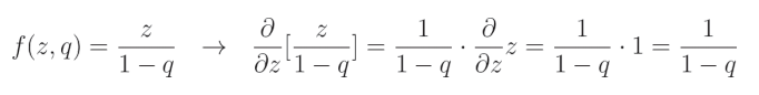
这是因为相对于 z z z 的导数 ∂ z ∂ z \frac{\partial z}{\partial z} ∂z∂z 等于1，而其余部分被视为常数。

当 r i = 0 r_i=0 ri=0 时：

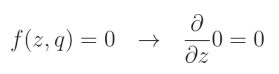
这是因为我们将 dropout 滤波器的这一元素置零，而任何常数值（包括0）的导数都是0。让我们将两种情况结合起来，并将 Dropout 表示为 D r Dr Dr：

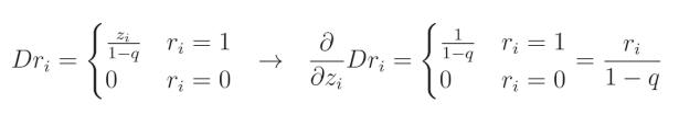
i i i 表示给定输入（以及层输出）的索引。当我们以这种方式写出 dropout 函数的导数时，可以将其简化为来自伯努利分布的值除以 1 − q 1-q 1−q，这与我们在前向传播中应用的缩放掩码相同，因为它同样是 1 1 1 除以 1 − q 1-q 1−q 或 0 0 0。因此，我们可以在前向传播期间保存这个掩码，并在链式法则中将其用作该函数的梯度。

3. 代码

现在，我们可以在一种新的层类型--dropout层--中实现这一概念：

# Dropout
class Layer_Dropout:
    # Init
    def __init__(self, rate):
        # Store rate, we invert it as for example for dropout
        # of 0.1 we need success rate of 0.9
        self.rate = 1 - rate
        
    # Forward pass
    def forward(self, inputs):
        # Save input values
        self.inputs = inputs
        # Generate and save scaled mask
        self.binary_mask = np.random.binomial(1, self.rate, size=inputs.shape) / self.rate
        # Apply mask to output values
        self.output = inputs * self.binary_mask
        
    # Backward pass
    def backward(self, dvalues):
        # Gradient on values
        self.dinputs = dvalues * self.binary_mask

让我们把这个新的滤色层添加到两个dense层之间。首先定义它：

# Create Dense layer with 2 input features and 64 output values
dense1 = Layer_Dense(2, 64, weight_regularizer_l2=5e-4, bias_regularizer_l2=5e-4)

# Create ReLU activation (to be used with Dense layer):
activation1 = Activation_ReLU()

# Create dropout layer
dropout1 = Layer_Dropout(0.1)

# Create second Dense layer with 64 input features (as we take output
# of previous layer here) and 3 output values (output values)
dense2 = Layer_Dense(64, 3)

在向前传递过程中，加入dropout：

# Perform a forward pass through Dropout layer
dropout1.forward(activation1.output)

# Perform a forward pass through second Dense layer
# takes outputs of activation function of first layer as inputs
dense2.forward(dropout1.output)

当然还有backward pass：

dropout1.backward(dense2.dinputs)
activation1.backward(dropout1.dinputs)

我们还可以稍微提高学习率，从0.02提升到0.05，同时将学习率衰减从 5 × 1 0 − 7 5 \times 10^{-7} 5×10−7提升到 5 × 1 0 − 5 5 \times 10^{-5} 5×10−5，因为这些参数更适合我们的模型和dropout层。

到目前为止的全部代码：

import numpy as np
import nnfs
from nnfs.datasets import spiral_data

nnfs.init()

# Dense layer
class Layer_Dense:
    # Layer initialization
    def __init__(self, n_inputs, n_neurons,
                 weight_regularizer_l1=0, weight_regularizer_l2=0,
                 bias_regularizer_l1=0, bias_regularizer_l2=0):
        # Initialize weights and biases
        self.weights = 0.01 * np.random.randn(n_inputs, n_neurons)
        self.biases = np.zeros((1, n_neurons))
        # Set regularization strength
        self.weight_regularizer_l1 = weight_regularizer_l1
        self.weight_regularizer_l2 = weight_regularizer_l2
        self.bias_regularizer_l1 = bias_regularizer_l1
        self.bias_regularizer_l2 = bias_regularizer_l2
        
    # Forward pass
    def forward(self, inputs):
        # Remember input values
        self.inputs = inputs
        # Calculate output values from inputs, weights and biases
        self.output = np.dot(inputs, self.weights) + self.biases
    
    # Backward pass
    def backward(self, dvalues):
        # Gradients on parameters
        self.dweights = np.dot(self.inputs.T, dvalues)
        self.dbiases = np.sum(dvalues, axis=0, keepdims=True)
        # Gradients on regularization
        # L1 on weights
        if self.weight_regularizer_l1 > 0:
            dL1 = np.ones_like(self.weights)
            dL1[self.weights < 0] = -1
            self.dweights += self.weight_regularizer_l1 * dL1
        # L2 on weights
        if self.weight_regularizer_l2 > 0:
            self.dweights += 2 * self.weight_regularizer_l2 * self.weights
        # L1 on biases
        if self.bias_regularizer_l1 > 0:
            dL1 = np.ones_like(self.biases)
            dL1[self.biases < 0] = -1
            self.dbiases += self.bias_regularizer_l1 * dL1
        # L2 on biases
        if self.bias_regularizer_l2 > 0:
            self.dbiases += 2 * self.bias_regularizer_l2 * self.biases
        # Gradient on values
        self.dinputs = np.dot(dvalues, self.weights.T)
        
        
# ReLU activation
class Activation_ReLU:        
        # Forward pass
        def forward(self, inputs):
            # Remember input values
            self.inputs = inputs
            # Calculate output values from inputs
            self.output = np.maximum(0, inputs)
        
        # Backward pass
        def backward(self, dvalues):
            # Since we need to modify original variable,
            # let's make a copy of values first
            self.dinputs = dvalues.copy()
            # Zero gradient where input values were negative
            self.dinputs[self.inputs <= 0] = 0
        
        
# Softmax activation
class Activation_Softmax:        
        # Forward pass
        def forward(self, inputs):
            # Remember input values
            self.inputs = inputs
            # Get unnormalized probabilities
            exp_values = np.exp(inputs - np.max(inputs, axis=1, keepdims=True))
            # Normalize them for each sample
            probabilities = exp_values / np.sum(exp_values, axis=1, keepdims=True)
            self.output = probabilities
        
        # Backward pass
        def backward(self, dvalues):
            # Create uninitialized array
            self.dinputs = np.empty_like(dvalues)
            # Enumerate outputs and gradients
            for index, (single_output, single_dvalues) in enumerate(zip(self.output, dvalues)):
                # Flatten output array
                single_output = single_output.reshape(-1, 1)
                # Calculate Jacobian matrix of the output and
                jacobian_matrix = np.diagflat(single_output) - np.dot(single_output, single_output.T)
                # Calculate sample-wise gradient
                # and add it to the array of sample gradients
                self.dinputs[index] = np.dot(jacobian_matrix, single_dvalues)
        
        
# SGD optimizer
class Optimizer_SGD:
    # Initialize optimizer - set settings,
    # learning rate of 1. is default for this optimizer
    def __init__(self, learning_rate=1., decay=0., momentum=0.):
        self.learning_rate = learning_rate
        self.current_learning_rate = learning_rate
        self.decay = decay
        self.iterations = 0
        self.momentum = momentum        
        
    # Call once before any parameter updates
    def pre_update_params(self):
        if self.decay:
            self.current_learning_rate = self.learning_rate * (1. / (1. + self.decay * self.iterations))
            
    # Update parameters
    def update_params(self, layer):        
        # If we use momentum
        if self.momentum:
            # If layer does not contain momentum arrays, create them
            # filled with zeros
            if not hasattr(layer, 'weight_momentums'):
                layer.weight_momentums = np.zeros_like(layer.weights)
                # If there is no momentum array for weights
                # The array doesn't exist for biases yet either.
                layer.bias_momentums = np.zeros_like(layer.biases)
            # Build weight updates with momentum - take previous
            # updates multiplied by retain factor and update with
            # current gradients
            weight_updates = self.momentum * layer.weight_momentums - self.current_learning_rate * layer.dweights
            layer.weight_momentums = weight_updates
            # Build bias updates
            bias_updates = self.momentum * layer.bias_momentums - self.current_learning_rate * layer.dbiases
            layer.bias_momentums = bias_updates
        # Vanilla SGD updates (as before momentum update)
        else:
            weight_updates = -self.current_learning_rate * layer.dweights
            bias_updates = -self.current_learning_rate * layer.dbiases
        # Update weights and biases using either
        # vanilla or momentum updates
        layer.weights += weight_updates
        layer.biases += bias_updates
     
    # Call once after any parameter updates
    def post_update_params(self):
        self.iterations += 1
        
        
# Adagrad optimizer
class Optimizer_Adagrad:
    # Initialize optimizer - set settings
    def __init__(self, learning_rate=1., decay=0., epsilon=1e-7):
        self.learning_rate = learning_rate
        self.current_learning_rate = learning_rate
        self.decay = decay
        self.iterations = 0
        self.epsilon = epsilon        
      
    # Call once before any parameter updates
    def pre_update_params(self):
        if self.decay:
            self.current_learning_rate = self.learning_rate * (1. / (1. + self.decay * self.iterations))
        
    # Update parameters
    def update_params(self, layer):
        # If layer does not contain cache arrays,
        # create them filled with zeros
        if not hasattr(layer, 'weight_cache'):
            layer.weight_cache = np.zeros_like(layer.weights)
            layer.bias_cache = np.zeros_like(layer.biases)
        # Update cache with squared current gradients
        layer.weight_cache += layer.dweights**2
        layer.bias_cache += layer.dbiases**2
        # Vanilla SGD parameter update + normalization
        # with square rooted cache
        layer.weights += -self.current_learning_rate * layer.dweights / (np.sqrt(layer.weight_cache) + self.epsilon)
        layer.biases += -self.current_learning_rate * layer.dbiases / (np.sqrt(layer.bias_cache) + self.epsilon)    
        
    # Call once after any parameter updates
    def post_update_params(self):
        self.iterations += 1        
        
        
# RMSprop optimizer
class Optimizer_RMSprop:        
    # Initialize optimizer - set settings
    def __init__(self, learning_rate=0.001, decay=0., epsilon=1e-7, rho=0.9):
        self.learning_rate = learning_rate
        self.current_learning_rate = learning_rate
        self.decay = decay
        self.iterations = 0
        self.epsilon = epsilon
        self.rho = rho    
    
    # Call once before any parameter updates
    def pre_update_params(self):
        if self.decay:
            self.current_learning_rate = self.learning_rate * (1. / (1. + self.decay * self.iterations))
    
    # Update parameters
    def update_params(self, layer):
        # If layer does not contain cache arrays,
        # create them filled with zeros
        if not hasattr(layer, 'weight_cache'):
            layer.weight_cache = np.zeros_like(layer.weights)
            layer.bias_cache = np.zeros_like(layer.biases)
        # Update cache with squared current gradients
        layer.weight_cache = self.rho * layer.weight_cache + (1 - self.rho) * layer.dweights**2
        layer.bias_cache = self.rho * layer.bias_cache + (1 - self.rho) * layer.dbiases**2
        # Vanilla SGD parameter update + normalization
        # with square rooted cache
        layer.weights += -self.current_learning_rate * layer.dweights / (np.sqrt(layer.weight_cache) + self.epsilon)
        layer.biases += -self.current_learning_rate * layer.dbiases / (np.sqrt(layer.bias_cache) + self.epsilon)
        
    # Call once after any parameter updates
    def post_update_params(self):
        self.iterations += 1
        
        
# Adam optimizer
class Optimizer_Adam:
    # Initialize optimizer - set settings
    def __init__(self, learning_rate=0.001, decay=0., epsilon=1e-7, beta_1=0.9, beta_2=0.999):
        self.learning_rate = learning_rate
        self.current_learning_rate = learning_rate
        self.decay = decay
        self.iterations = 0
        self.epsilon = epsilon
        self.beta_1 = beta_1
        self.beta_2 = beta_2        
        
    # Call once before any parameter updates
    def pre_update_params(self):
        if self.decay:
            self.current_learning_rate = self.learning_rate * (1. / (1. + self.decay * self.iterations))
        
    # Update parameters
    def update_params(self, layer):
        # If layer does not contain cache arrays,
        # create them filled with zeros
        if not hasattr(layer, 'weight_cache'):
            layer.weight_momentums = np.zeros_like(layer.weights)
            layer.weight_cache = np.zeros_like(layer.weights)
            layer.bias_momentums = np.zeros_like(layer.biases)
            layer.bias_cache = np.zeros_like(layer.biases)
        # Update momentum with current gradients
        layer.weight_momentums = self.beta_1 * layer.weight_momentums + (1 - self.beta_1) * layer.dweights
        layer.bias_momentums = self.beta_1 * layer.bias_momentums + (1 - self.beta_1) * layer.dbiases
        # Get corrected momentum
        # self.iteration is 0 at first pass
        # and we need to start with 1 here
        weight_momentums_corrected = layer.weight_momentums / (1 - self.beta_1 ** (self.iterations + 1))
        bias_momentums_corrected = layer.bias_momentums / (1 - self.beta_1 ** (self.iterations + 1))
        # Update cache with squared current gradients
        layer.weight_cache = self.beta_2 * layer.weight_cache + (1 - self.beta_2) * layer.dweights**2
        layer.bias_cache = self.beta_2 * layer.bias_cache + (1 - self.beta_2) * layer.dbiases**2
        # Get corrected cache
        weight_cache_corrected = layer.weight_cache / (1 - self.beta_2 ** (self.iterations + 1))
        bias_cache_corrected = layer.bias_cache / (1 - self.beta_2 ** (self.iterations + 1))
        # Vanilla SGD parameter update + normalization
        # with square rooted cache
        layer.weights += -self.current_learning_rate * weight_momentums_corrected / (np.sqrt(weight_cache_corrected) + self.epsilon)
        layer.biases += -self.current_learning_rate * bias_momentums_corrected / (np.sqrt(bias_cache_corrected) + self.epsilon)
        
    # Call once after any parameter updates
    def post_update_params(self):
        self.iterations += 1


# Common loss class
class Loss:        
    # Regularization loss calculation
    def regularization_loss(self, layer):
        # 0 by default
        regularization_loss = 0
        # L1 regularization - weights
        # calculate only when factor greater than 0
        if layer.weight_regularizer_l1 > 0:
            regularization_loss += layer.weight_regularizer_l1 * np.sum(np.abs(layer.weights))
        # L2 regularization - weights
        if layer.weight_regularizer_l2 > 0:
            regularization_loss += layer.weight_regularizer_l2 * np.sum(layer.weights * layer.weights)
        # L1 regularization - biases
        # calculate only when factor greater than 0
        if layer.bias_regularizer_l1 > 0:
            regularization_loss += layer.bias_regularizer_l1 * np.sum(np.abs(layer.biases))
        # L2 regularization - biases
        if layer.bias_regularizer_l2 > 0:
            regularization_loss += layer.bias_regularizer_l2 * np.sum(layer.biases * layer.biases)
        return regularization_loss
    
    # Calculates the data and regularization losses
    # given model output and ground truth values
    def calculate(self, output, y):
        # Calculate sample losses
        sample_losses = self.forward(output, y)
        # Calculate mean loss
        data_loss = np.mean(sample_losses)
        # Return loss
        return data_loss
        
        
# Cross-entropy loss
class Loss_CategoricalCrossentropy(Loss):
    # Forward pass
    def forward(self, y_pred, y_true):
        # Number of samples in a batch
        samples = len(y_pred)
        # Clip data to prevent division by 0
        # Clip both sides to not drag mean towards any value
        y_pred_clipped = np.clip(y_pred, 1e-7, 1 - 1e-7)
        # Probabilities for target values -
        # only if categorical labels
        if len(y_true.shape) == 1:
            correct_confidences = y_pred_clipped[range(samples), y_true]        
        # Mask values - only for one-hot encoded labels
        elif len(y_true.shape) == 2:
            correct_confidences = np.sum(y_pred_clipped * y_true, axis=1)
        # Losses
        negative_log_likelihoods = -np.log(correct_confidences)
        return negative_log_likelihoods
        
    # Backward pass
    def backward(self, dvalues, y_true):
        # Number of samples
        samples = len(dvalues)
        # Number of labels in every sample
        # We'll use the first sample to count them
        labels = len(dvalues[0])
        # If labels are sparse, turn them into one-hot vector
        if len(y_true.shape) == 1:
            y_true = np.eye(labels)[y_true]
        # Calculate gradient
        self.dinputs = -y_true / dvalues
        # Normalize gradient
        self.dinputs = self.dinputs / samples
        
        
# Softmax classifier - combined Softmax activation
# and cross-entropy loss for faster backward step
class Activation_Softmax_Loss_CategoricalCrossentropy():
    # Creates activation and loss function objects
    def __init__(self):
        self.activation = Activation_Softmax()
        self.loss = Loss_CategoricalCrossentropy()
        
    # Forward pass
    def forward(self, inputs, y_true):
        # Output layer's activation function
        self.activation.forward(inputs)
        # Set the output
        self.output = self.activation.output
        # Calculate and return loss value
        return self.loss.calculate(self.output, y_true)        
        
    # Backward pass
    def backward(self, dvalues, y_true):
        # Number of samples
        samples = len(dvalues)
        # If labels are one-hot encoded,
        # turn them into discrete values
        if len(y_true.shape) == 2:
            y_true = np.argmax(y_true, axis=1)
        # Copy so we can safely modify
        self.dinputs = dvalues.copy()
        # Calculate gradient
        self.dinputs[range(samples), y_true] -= 1
        # Normalize gradient
        self.dinputs = self.dinputs / samples
        
        
# Dropout
class Layer_Dropout:
    # Init
    def __init__(self, rate):
        # Store rate, we invert it as for example for dropout
        # of 0.1 we need success rate of 0.9
        self.rate = 1 - rate
        
    # Forward pass
    def forward(self, inputs):
        # Save input values
        self.inputs = inputs
        # Generate and save scaled mask
        self.binary_mask = np.random.binomial(1, self.rate, size=inputs.shape) / self.rate
        # Apply mask to output values
        self.output = inputs * self.binary_mask
        
    # Backward pass
    def backward(self, dvalues):
        # Gradient on values
        self.dinputs = dvalues * self.binary_mask

        
        
# Create dataset
X, y = spiral_data(samples=1000, classes=3)

# Create Dense layer with 2 input features and 64 output values
# dense1 = Layer_Dense(2, 64, weight_regularizer_l2=5e-4, bias_regularizer_l2=5e-4)  
# dense1 = Layer_Dense(2, 256, weight_regularizer_l2=5e-4, bias_regularizer_l2=5e-4)  
dense1 = Layer_Dense(2, 64, weight_regularizer_l2=5e-4, bias_regularizer_l2=5e-4)        
        
# Create ReLU activation (to be used with Dense layer):
activation1 = Activation_ReLU()

# Create dropout layer
dropout1 = Layer_Dropout(0.1)

# Create second Dense layer with 64 input features (as we take output
# of previous layer here) and 3 output values (output values)
# dense2 = Layer_Dense(64, 3)
# dense2 = Layer_Dense(256, 3)
dense2 = Layer_Dense(64, 3)

# Create Softmax classifier's combined loss and activation
loss_activation = Activation_Softmax_Loss_CategoricalCrossentropy()

# Create optimizer
optimizer = Optimizer_Adam(learning_rate=0.05, decay=5e-5)        
        
# Train in loop
for epoch in range(10001):
    # Perform a forward pass of our training data through this layer
    dense1.forward(X)
    
    # Perform a forward pass through activation function
    # takes the output of first dense layer here
    activation1.forward(dense1.output)     
    
    # Perform a forward pass through Dropout layer
    dropout1.forward(activation1.output)

    # Perform a forward pass through second Dense layer
    # takes outputs of activation function of first layer as inputs
    dense2.forward(activation1.output)
    
    # Perform a forward pass through the activation/loss function
    # takes the output of second dense layer here and returns loss
    data_loss = loss_activation.forward(dense2.output, y)
    
    # Calculate regularization penalty
    regularization_loss = loss_activation.loss.regularization_loss(dense1) + loss_activation.loss.regularization_loss(dense2)
    
    # Calculate overall loss
    loss = data_loss + regularization_loss
    
    # Calculate accuracy from output of activation2 and targets
    # calculate values along first axis
    predictions = np.argmax(loss_activation.output, axis=1)
    if len(y.shape) == 2:
        y = np.argmax(y, axis=1)
    accuracy = np.mean(predictions==y)
    
    if not epoch % 100:
        print(f'epoch: {epoch}, ' +
              f'acc: {accuracy:.3f}, ' +
              f'loss: {loss:.3f} (' +
              f'data_loss: {data_loss:.3f}, ' +
              f'reg_loss: {regularization_loss:.3f}), ' +
              f'lr: {optimizer.current_learning_rate}')
        
    # Backward pass
    loss_activation.backward(loss_activation.output, y)
    dense2.backward(loss_activation.dinputs)
    dropout1.backward(dense2.dinputs)
    activation1.backward(dense2.dinputs)
    dense1.backward(activation1.dinputs)
    
    # Update weights and biases
    optimizer.pre_update_params()
    optimizer.update_params(dense1)
    optimizer.update_params(dense2)
    optimizer.post_update_params()
        
# Validate the model
# Create test dataset
X_test, y_test = spiral_data(samples=100, classes=3)

# Perform a forward pass of our testing data through this layer
dense1.forward(X_test)

# Perform a forward pass through activation function
# takes the output of first dense layer here
activation1.forward(dense1.output)

# Perform a forward pass through second Dense layer
# takes outputs of activation function of first layer as inputs
dense2.forward(activation1.output)

# Perform a forward pass through the activation/loss function
# takes the output of second dense layer here and returns loss
loss = loss_activation.forward(dense2.output, y_test)

# Calculate accuracy from output of activation2 and targets
# calculate values along first axis
predictions = np.argmax(loss_activation.output, axis=1)
if len(y_test.shape) == 2:
    y_test = np.argmax(y_test, axis=1)
accuracy = np.mean(predictions==y_test)

print(f'validation, acc: {accuracy:.3f}, loss: {loss:.3f}')        

>>>
epoch: 9900, acc: 0.913, loss: 0.278 (data_loss: 0.230, reg_loss: 0.048), lr: 0.0334459346466437
epoch: 10000, acc: 0.915, loss: 0.277 (data_loss: 0.230, reg_loss: 0.048), lr: 0.03333444448148271
validation, acc: 0.910, loss: 0.240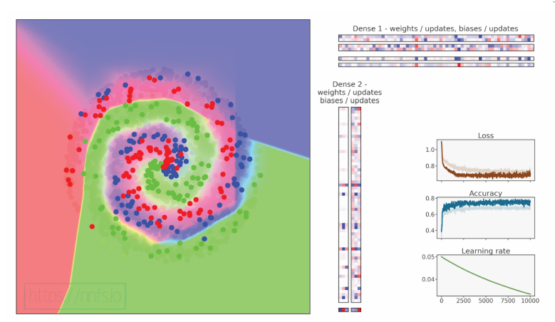

代码可视化：https://nnfs.io/efg

虽然我们的准确率和损失显著下降，但我们发现了一种验证集比训练集表现更好的情况（因为在测试时并未应用 dropout，因此不会禁用部分连接）。进一步调整可能会解决准确率问题；例如，由于我们的正则化策略，我们可以将层的大小更改为 512：

# Create Dense layer with 2 input features and 512 output values
dense1 = Layer_Dense(2, 512, weight_regularizer_l2=5e-4, bias_regularizer_l2=5e-4)

# Create ReLU activation (to be used with Dense layer):
activation1 = Activation_ReLU()

# Create dropout layer
dropout1 = Layer_Dropout(0.1)

# Create second Dense layer with 512 input features
# and 3 output values
dense2 = Layer_Dense(512, 3)

>>>
epoch: 0, acc: 0.373, loss: 1.099 (data_loss: 1.099, reg_loss: 0.000), lr:
0.05
epoch: 100, acc: 0.719, loss: 0.735 (data_loss: 0.672, reg_loss: 0.063), lr:
0.04975371909050202
epoch: 200, acc: 0.782, loss: 0.627 (data_loss: 0.548, reg_loss: 0.079), lr:
0.049507401356502806
epoch: 300, acc: 0.800, loss: 0.603 (data_loss: 0.521, reg_loss: 0.082), lr:
0.0492635105177595
epoch: 400, acc: 0.802, loss: 0.595 (data_loss: 0.513, reg_loss: 0.082), lr:
0.04902201088288642
epoch: 500, acc: 0.809, loss: 0.562 (data_loss: 0.482, reg_loss: 0.079), lr:
0.048782867456949125
epoch: 600, acc: 0.836, loss: 0.521 (data_loss: 0.445, reg_loss: 0.076), lr:
0.04854604592455945
epoch: 700, acc: 0.816, loss: 0.532 (data_loss: 0.457, reg_loss: 0.076), lr:
0.048311512633460556
epoch: 800, acc: 0.839, loss: 0.515 (data_loss: 0.442, reg_loss: 0.073), lr:
0.04807923457858551
epoch: 900, acc: 0.842, loss: 0.499 (data_loss: 0.426, reg_loss: 0.072), lr:
0.04784917938657352
epoch: 1000, acc: 0.837, loss: 0.480 (data_loss: 0.408, reg_loss: 0.071),
lr: 0.04762131530072861
...
epoch: 9800, acc: 0.848, loss: 0.443 (data_loss: 0.391, reg_loss: 0.052),
lr: 0.033558173093056816
epoch: 9900, acc: 0.841, loss: 0.468 (data_loss: 0.416, reg_loss: 0.052),
lr: 0.0334459346466437
epoch: 10000, acc: 0.859, loss: 0.468 (data_loss: 0.417, reg_loss: 0.051),
lr: 0.03333444448148271
validation, acc: 0.857, loss: 0.397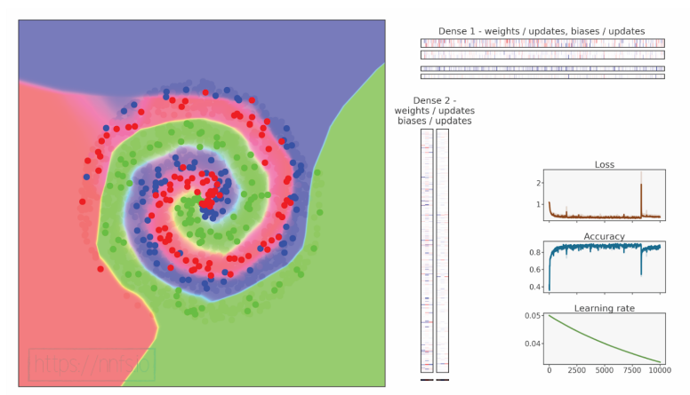

代码可视化：https://nnfs.io/fgh

结果还不错，但相比于"无dropout"模型稍差。有趣的是，使用dropout的情况下，验证精度接近训练精度------通常验证精度会更高，因此我们可能怀疑这里存在过拟合的迹象（验证损失低于预期）。

---

本章的章节代码、更多资源和勘误表：https://nnfs.io/ch15