042_Unscented Kalman Filter in Matlab无迹卡尔曼滤波

无迹卡尔曼滤波(Unscented Kalman Filter, UKF)

无迹卡尔曼滤波(Unscented Kalman Filter, UKF)是一种基于卡尔曼滤波的非线性状态估计方法，它通过一种称为无迹变换(Unscented Transformation)的方法，将非线性系统的状态估计问题转化为线性系统的状态估计问题，然后使用卡尔曼滤波器进行状态估计。

这是一种在线方法，也就是说，它会连续地对系统状态进行估计，而不是像批处理方法那样，一次性处理所有的数据。

要定义一个UKF，我们需要定义如下两个函数：

状态转移函数 f ( x , u , t ) f(x, u, t) f(x,u,t)
观测函数 h ( x ) h(x) h(x)

其中， x x x 是状态向量， u u u 是控制向量， t t t 是时间， f f f 是状态转移函数， h h h 是观测函数。

提供这两个函数外加噪声的信息，既可以创建一个UKF对象。其后，就可以通过predict来预测下个时间步长的状态；在拿到实时数据后，通过correct函数来校正状态。

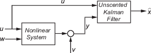
系统的框图如上所示。非线性系统的输入为 u u u，系统噪声为 w w w，系统状态为 x x x，观测值为 y y y，观测噪声为 v v v。UKF 通过输入 u u u 和观测值 y y y 来估计系统状态 x ^ \hat{x} x^。

van der Pol Oscillator

这里我们以 van der Pol Oscillator 为例，来演示如何使用 UKF 进行状态估计。

首先，我们给出 van der Pol Oscillator 的一般形式：

x ¨ − μ ( 1 − x 2 ) x ˙ + x = 0 \ddot{x} - \mu (1 - x^2) \dot{x} + x = 0 x¨−μ(1−x2)x˙+x=0

其中， μ \mu μ 是 van der Pol Oscillator 的参数。

这个方程可以被转化为两个一阶微分方程：

{ x 1 ˙ = x 2 x 2 ˙ = μ ( 1 − x 1 2 ) x 2 − x 1 \begin{cases} \dot{x_1} &= x_2 \\\\ \dot{x_2} &= \mu (1 - x_1^2) x_2 - x_1 \\\\ \end{cases} ⎩ ⎨ ⎧x1˙x2˙=x2=μ(1−x12)x2−x1

采用ODE45求解这个方程，我们可以得到 van der Pol Oscillator 的状态变化。

matlab 复制代码

T = 0.05; % [s] Filter sample time
timeVector = 0:T:5;
[t, xTrue] = ode45(@vdp1, timeVector, [2; 0]);

figure;
plot(t, xTrue, 'LineWidth', 2);
xlabel('Time [s]');
ylabel('States');
legend('x_1', 'x_2', 'Location', 'Best');
title('Van der Pol Oscillator');
grid on;

exportgraphics(gcf, '../matlab-img/vdp1Ode.png', 'Resolution', 100);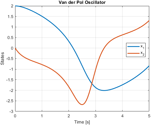

观测

假设我们对 van der Pol Oscillator 的状态进行观测，但是观测值是带有噪声的。

{ R = 0.2 y 1 = x 1 ∗ ( 1 + N ( 0 , R ) ) \begin{cases} R = 0.2 \\\\ y_1 = x_1 * (1 + \mathcal{N}(0, R)) \\\\ \end{cases} ⎩ ⎨ ⎧R=0.2y1=x1∗(1+N(0,R))

matlab 复制代码

R = 0.2;

rng(1); % For reproducibility
yTrue = xTrue(:, 1);
yMeas = yTrue .* (1 + sqrt(R) * randn(size(yTrue)));

figure;
plot(t, yTrue, 'LineWidth', 2);
hold on;
plot(t, yMeas, 'LineWidth', 2);
xlabel('Time [s]');
ylabel('State: x_1');
legend('True', 'Measured', 'Location', 'Best');
title('Van der Pol Oscillator Observations of x_1');

exportgraphics(gcf, '../matlab-img/vdp1Observ.png', 'Resolution', 100);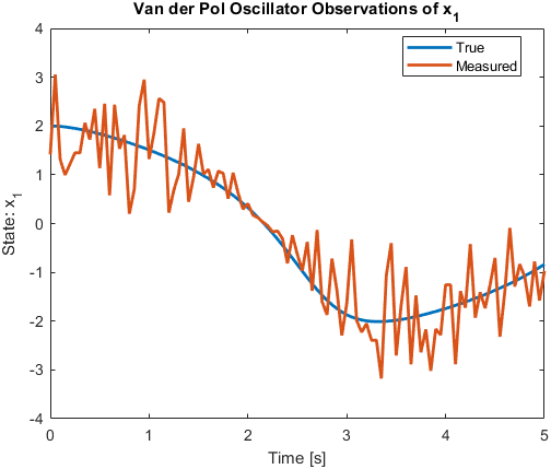

UKF

接下来，我们使用 UKF 对 van der Pol Oscillator 的状态进行估计。

matlab 复制代码

% 猜测初始状态
initialStateGuess = [2; 0]; % xhat[k|k-1]
% 构造 UKF
ukf = unscentedKalmanFilter( ...
    @vdpStateFcn, ... % State transition function
    @vdpMeasurementNonAdditiveNoiseFcn, ... % Measurement function
    initialStateGuess, ...
    'HasAdditiveMeasurementNoise', false);

% 设置 UKF 参数
ukf.MeasurementNoise = R;
ukf.ProcessNoise = diag([0.02 0.1]);

% 初始化数组存储
Nsteps = numel(yMeas); % Number of time steps
xCorrectedUKF = zeros(Nsteps, 2); % Corrected state estimates
PCorrected = zeros(Nsteps, 2, 2); % Corrected state estimation error covariances
e = zeros(Nsteps, 1); % Residuals (or innovations)

for k = 1:Nsteps % k时刻
    % 新息更新
    e(k) = yMeas(k) - vdpMeasurementFcn(ukf.State); % ukf.State <- x[k|k-1]
    % 新的输入测量更新状态估计
    [xCorrectedUKF(k, :), PCorrected(k, :, :)] = correct(ukf, yMeas(k)); % ukf.State <- x[k|k]
    % 预测下一个状态
    predict(ukf);
end

% 绘制结果
figure();
h = plot(timeVector, xTrue(:, 1), timeVector, xCorrectedUKF(:, 1), timeVector, yMeas(:), 'LineWidth', 0.5);
set(h(2), 'LineWidth', 2);
set(h(1), 'LineWidth', 2);

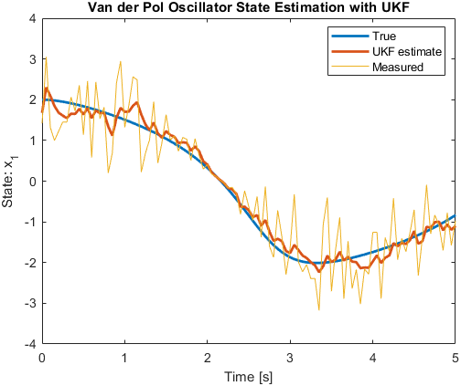
legend('True', 'UKF estimate', 'Measured', 'Location', 'Best');
xlabel('Time [s]');
ylabel('State: x_1');
title('Van der Pol Oscillator State Estimation with UKF');

exportgraphics(gcf, '../matlab-img/vdp1Ukf.png', 'Resolution', 100);

function x = vdpStateFcn(x)
    dt = 0.05; % [s] Sample time
    x = x + vdpStateFcnContinuous(x) * dt;
end

function dxdt = vdpStateFcnContinuous(x)
    %取 mu = 1的 van der Pol ODE
    dxdt = [x(2); (1 - x(1) ^ 2) * x(2) - x(1)];
end

function yk = vdpMeasurementNonAdditiveNoiseFcn(xk, vk)
    yk = xk(1) * (1 + vk);
end

经过 UKF 估计后，我们可以得到 van der Pol Oscillator 的状态估计值。

进一步分析

当然，我们还可以对新息、协方差等进行分析。这里仅仅展示对一个连续的状态进行UKF估计的过程。

参考：Van der Pol Equation: Overview, Derivation, and Examination of Solutions