torch.einsum 的 10 个常见用法详解以及多头注意力实现

torch.einsum 是 PyTorch 提供的一个高效的张量运算函数，能够用紧凑的 Einstein Summation 约定（Einstein Summation Convention, Einsum）描述复杂的张量操作，例如矩阵乘法、转置、内积、外积、批量矩阵乘法等。

1. 基本语法

python 复制代码

torch.einsum(equation, *operands)

• equation：爱因斯坦求和表示法的字符串，例如 "ij,jk->ik"

• operands：参与计算的张量，可以是多个

2. 基本概念

Einsum 使用 -> 将输入与输出模式分开：

• 左侧：表示输入张量的索引

• 右侧：表示输出张量的索引

• 省略求和索引：会自动对省略的索引进行求和（即 Einstein Summation 规则）

3. torch.einsum 的 10 个常见用法

(1) 矩阵乘法 (torch.mm)

python 复制代码

import torch

A = torch.randn(2, 3)
B = torch.randn(3, 4)

C = torch.einsum("ij,jk->ik", A, B)  # 矩阵乘法
print(C.shape)  # torch.Size([2, 4])

解析：

• ij 表示 A 的形状 (2,3)

• jk 表示 B 的形状 (3,4)

• 由于 j 在 -> 右侧没有出现，因此对其求和，最终得到形状 (2,4)

(2) 向量点积 (torch.dot)

python 复制代码

a = torch.tensor([1, 2, 3])
b = torch.tensor([4, 5, 6])

dot_product = torch.einsum("i,i->", a, b)  # 向量点积
print(dot_product)  # 输出: 32

解析：

• i,i-> 代表对应位置相乘并求和，等价于 torch.dot(a, b)

(3) 矩阵转置 (torch.transpose)

python 复制代码

A = torch.randn(2, 3)

A_T = torch.einsum("ij->ji", A)  # 矩阵转置
print(A_T.shape)  # torch.Size([3, 2])

解析：

• ij->ji 交换 i 和 j 维度，相当于 A.T

(4) 矩阵外积 (torch.outer)

python 复制代码

a = torch.tensor([1, 2, 3])
b = torch.tensor([4, 5, 6])

outer_product = torch.einsum("i,j->ij", a, b)  # 外积
print(outer_product)
# tensor([[ 4,  5,  6],
#         [ 8, 10, 12],
#         [12, 15, 18]])

解析：

• i,j->ij 生成形状 (3,3) 的矩阵

(5) 批量矩阵乘法 (torch.bmm)

python 复制代码

A = torch.randn(5, 2, 3)
B = torch.randn(5, 3, 4)

C = torch.einsum("bij,bjk->bik", A, B)  # 批量矩阵乘法
print(C.shape)  # torch.Size([5, 2, 4])

解析：

• b 代表 batch 维度，不求和，保持

• j 出现在两个输入中但未出现在输出中，所以对其求和

(6) 计算均值 (torch.mean)

python 复制代码

A = torch.randn(3, 4)

mean_A = torch.einsum("ij->", A) / A.numel()  # 计算均值
print(mean_A)

解析：

• ij-> 表示所有元素求和

• A.numel() 是总元素数，等价于 torch.mean(A)

(7) 计算范数 (torch.norm)

python 复制代码

A = torch.randn(3, 4)

norm_A = torch.einsum("ij,ij->", A, A).sqrt()  # Frobenius 范数
print(norm_A)

解析：

• ij,ij-> 表示 A 的所有元素平方求和

• .sqrt() 计算范数

(8) 计算 Softmax

python 复制代码

A = torch.randn(3, 4)

softmax_A = torch.einsum("ij->ij", torch.exp(A)) / torch.einsum("ij->i1", torch.exp(A))
print(softmax_A)

解析：

• torch.exp(A) 计算指数

• torch.einsum("ij->i1", torch.exp(A)) 计算行和

(9) 对角线提取 (torch.diagonal)

python 复制代码

A = torch.randn(3, 3)

diag_A = torch.einsum("ii->i", A)  # 提取主对角线
print(diag_A)

解析：

• ii->i 只保留对角线元素，等价于 torch.diagonal(A)

(10) 计算张量 Hadamard 积（逐元素乘法）

python 复制代码

A = torch.randn(3, 4)
B = torch.randn(3, 4)

hadamard_product = torch.einsum("ij,ij->ij", A, B)  # 逐元素乘法
print(hadamard_product)

解析：

• ij,ij->ij 表示对相同索引位置元素相乘

总结

Einsum 公式	作用	等价 PyTorch 代码
`ij,jk->ik`	矩阵乘法	`torch.mm(A, B)`
`i,i->`	向量点积	`torch.dot(a, b)`
`i,j->ji`	矩阵转置	`A.T`
`bij,bjk->bik`	批量矩阵乘法	`torch.bmm(A, B)`
`ii->`	提取对角线	`torch.diagonal(A)`
`ij->`	矩阵所有元素求和	`A.sum()`
`ij,ij->ij`	Hadamard 乘法	`A * B`
`ij,ij->`	Frobenius 范数的平方	`(A**2).sum()`

使用 torch.einsum 计算多头注意力中的点积相似性

下面的代码示例演示如何使用 PyTorch 的 torch.einsum 函数来计算 Transformer 多头注意力机制中的点积注意力分数和输出。代码包含以下步骤：

定义输入 Q, K, V ：随机初始化查询（Query）、键（Key）、值（Value）张量，形状符合多头注意力的规范（包含 batch 维度和多头维度）。
计算 QK^T / sqrt(d_k) ：使用 torch.einsum 计算每个注意力头的 Q 与 K 转置的点积相似性，并除以 d k \sqrt{d_k} dk （注意力头维度的平方根）进行缩放。
计算 softmax 注意力权重 ：对第2步得到的相似性分数应用 softmax（在最后一个维度上），得到注意力权重分布。
计算最终的注意力输出 ：将 softmax 得到的注意力权重与值 V 相乘（加权求和）得到每个头的输出。
完整代码注释 ：代码中包含详尽的注释，解释每一步的用途。
可视化注意力权重 ：使用 Matplotlib 可视化一个头的注意力权重矩阵，以便更好地理解注意力分布。
具体参数设置：在代码开头指定 batch_size、sequence_length、embedding_dim、num_heads 等参数，便于调整。

python 复制代码

import torch
import torch.nn.functional as F
import math
import numpy as np
import matplotlib.pyplot as plt

# 7. 参数设置：定义 batch 大小、序列长度、嵌入维度、注意力头数等
batch_size = 2           # 批处理大小
sequence_length = 5      # 序列长度（假设查询和键序列长度相同）
embedding_dim = 16       # 整体嵌入维度（embedding维度）
num_heads = 4            # 注意力头数量
head_dim = embedding_dim // num_heads  # 每个注意力头的维度 d_k（需保证能够整除）

# 1. 定义输入 Q, K, V 张量（随机初始化）
# 形状约定：[batch_size, num_heads, seq_len, head_dim]
Q = torch.randn(batch_size, num_heads, sequence_length, head_dim)
K = torch.randn(batch_size, num_heads, sequence_length, head_dim)
V = torch.randn(batch_size, num_heads, sequence_length, head_dim)

# 打印 Q, K, V 的形状以验证
print("Q shape:", Q.shape)  # 预期: (batch_size, num_heads, sequence_length, head_dim)
print("K shape:", K.shape)  # 预期: (batch_size, num_heads, sequence_length, head_dim)
print("V shape:", V.shape)  # 预期: (batch_size, num_heads, sequence_length, head_dim)

# 2. 计算 QK^T / sqrt(d_k)
# 使用 torch.einsum 进行张量乘法：
# 'b h q d, b h k d -> b h q k' 表示：
#  - b: batch维度
#  - h: 多头维度
#  - q: 查询序列长度维度
#  - k: 键序列长度维度
#  - d: 每个头的维度（将对该维度进行求和，相当于点积）
# Q 的形状是 [b, h, q, d]，K 的形状是 [b, h, k, d]。
# einsum 根据 'd' 维度对 Q 和 K 相乘并求和，输出形状 [b, h, q, k]，即每个头的 Q 与每个 K 的点积。
scores = torch.einsum('b h q d, b h k d -> b h q k', Q, K)  # 点积 Q * K^T (尚未除以 sqrt(d_k))
scores = scores / math.sqrt(head_dim)  # 缩放除以 sqrt(d_k)

# 3. 计算 softmax 注意力权重
# 对最后一个维度 k 应用 softmax，得到注意力权重矩阵 (对每个 query位置，在所有 key位置上的权重分布和为1)
attention_weights = F.softmax(scores, dim=-1)

# 打印注意力权重矩阵的形状以验证
print("Attention weights shape:", attention_weights.shape)  # 预期: (batch_size, num_heads, seq_len, seq_len)

# 4. 计算最终的注意力输出
# 将注意力权重矩阵与值 V 相乘，得到每个查询位置的加权值。
# 我们再次使用 einsum：
# 'b h q k, b h k d -> b h q d' 表示：
#  - 将 attention_weights [b, h, q, k] 与 V [b, h, k, d] 在 k 维相乘并对 k 求和，
#    得到输出形状 [b, h, q, d]（每个头针对每个查询位置输出一个长度为d的向量）。
attention_output = torch.einsum('b h q k, b h k d -> b h q d', attention_weights, V)

# （可选）如果需要将多头的输出合并为一个张量，可以进一步 reshape/transpose 
# 并通过线性层投影。但这里我们仅关注多头内部的注意力计算。
# 合并示例: 将 out 从 [b, h, q, d] 变形为 [b, q, h*d]，再通过线性层投影回 [b, q, embedding_dim]。
combined_output = attention_output.permute(0, 2, 1, 3).reshape(batch_size, sequence_length, -1)
# 上面这行代码将 [b, h, q, d] 先变为 [b, q, h, d]，再合并h和d维度为[h*d]。
print("Combined output shape (after concatenating heads):", combined_output.shape)
# 注意：combined_output 的最后一维大小应当等于 embedding_dim（num_heads * head_dim）。

# 打印一个注意力输出张量的示例值（比如第一个 batch，第一头，第一查询位置的输出向量）
print("Sample attention output (batch 0, head 0, query 0):", attention_output[0, 0, 0])

# 5. 完整代码注释已在上方各步骤体现。

# 6. 可视化注意力权重
# 我们以第一个样本(batch 0)的第一个注意力头(head 0)的注意力权重矩阵为例进行可视化。
# 这个矩阵形状为 [seq_len, seq_len]，其中每行表示查询位置，每列表示键位置。
attn_matrix = attention_weights[0, 0].detach().numpy()  # 取出 batch 0, head 0 的注意力权重矩阵并转换为 numpy

plt.figure(figsize=(5,5))
plt.imshow(attn_matrix, cmap='viridis', origin='upper')
plt.colorbar()
plt.title("Attention Weights (Head 0 of Batch 0)")
plt.xlabel("Key position")
plt.ylabel("Query position")
plt.show()

运行上述代码后，您将看到打印的张量形状和示例值，以及一幅可视化的注意力权重热力图。图中纵轴为查询序列的位置，横轴为键序列的位置，颜色越亮表示注意力权重越高。通过该示例，您可以直观理解多头注意力机制中各查询对不同键"关注"的程度。

输出：

python 复制代码

Q shape: torch.Size([2, 4, 5, 4])
K shape: torch.Size([2, 4, 5, 4])
V shape: torch.Size([2, 4, 5, 4])
Attention weights shape: torch.Size([2, 4, 5, 5])
Combined output shape (after concatenating heads): torch.Size([2, 5, 16])
Sample attention output (batch 0, head 0, query 0): tensor([-0.8224, -1.1715, -0.0423, -0.0106])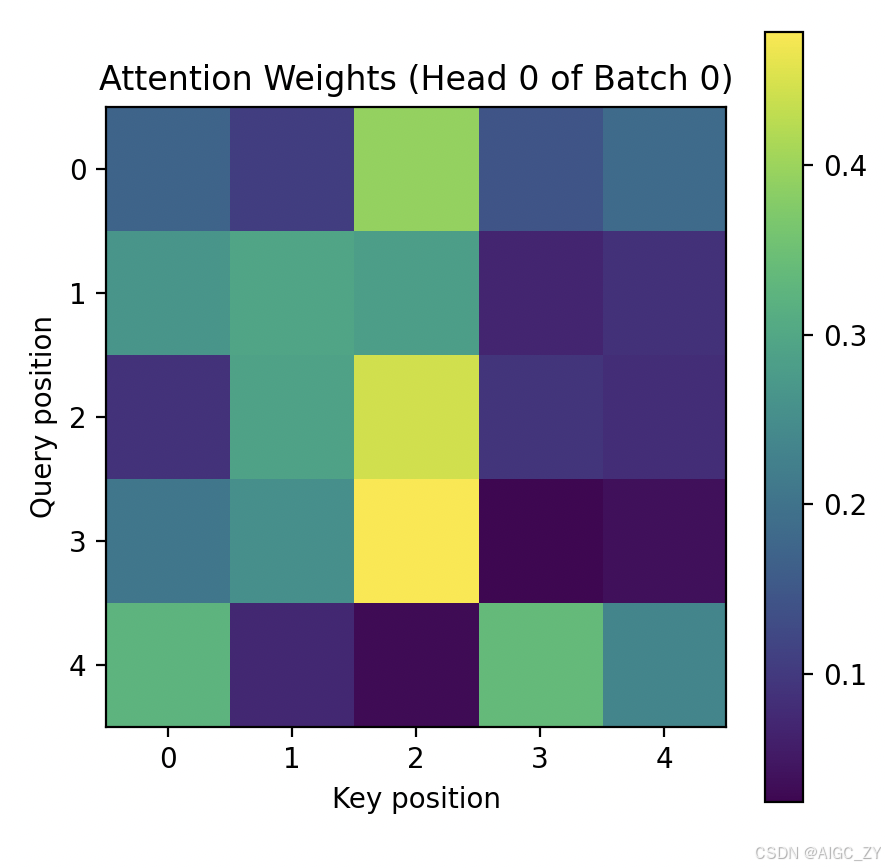

多头部分的计算：

python 复制代码

import torch

# 定义多头注意力机制的点积计算函数
def compute_attention_scores(queries, keys):
    # 计算点积相似性分数
    energy = torch.einsum("nqhd,nkhd->nhqk", [queries, keys])
    return energy

# 示例数据
N = 1            # 批次大小
q = 2            # 查询序列长度
k = 3            # 键序列长度
h = 2            # 注意力头数量
d = 4            # 每个注意力头的维度

# 随机生成 queries 和 keys
queries = torch.rand((N, q, h, d))  # Shape (1, 2, 2, 4)
keys = torch.rand((N, k, h, d))    # Shape (1, 3, 2, 4)

# 计算注意力分数
energy = compute_attention_scores(queries, keys)

print("Energy shape:", energy.shape)
print(energy)

输出
# Energy shape: torch.Size([1, 2, 2, 3])
# tensor([[[[0.7102, 0.3867, 0.5860],
#           [0.9586, 0.5920, 0.6626]],

#          [[1.3163, 0.9486, 0.5482],
#           [1.0403, 0.4555, 0.3656]]]])

更多资料：
torch.einsum用法详解

多头注意力：torch.einsum详解
 一文学会 Pytorch 中的 einsum
Python广播机制