🔥轨迹规划领域的 "YYDS"------minimum snap!作为基于优化的二次规划经典,它是无人机、自动驾驶轨迹规划论文必引的 "开山之作"。从优化目标函数到变量曲线表达,各路大神疯狂 "魔改",衍生出无数创新方案。
💡深度剖析百度 Apollo 的迭代奥秘:早期五次多项式拼接,如今离散点 piecewise jerk 路径 / 速度规划,本质皆是 minimum snap 的 "变形记"。
🚀想知道这些 "神操作" 背后的数学逻辑与技术细节?想解锁轨迹规划的优化新姿势?速来围观,带你直击前沿技术内核,开启轨迹规划的 "脑洞大开" 之旅!
问题:局部路径在运行的过程中对当下的速度和加速度进行采样,得到一个经过速度和加速度优化的轨迹进行运行是非常必要的,可以减少无人机单单用基于位置的简单的路径在空中经过PID或者其他控制以后出现振荡与大量抖动,这部分与控制并无关系,因为是期望都会不稳定,所以需要MinumSnap采用最小加加加速度(snap)的方法进行优化轨迹生成。
Fast-planner的全局规划主函数:
cpp
// 全局轨迹规划主函数,输入参数为起始位置
bool FastPlannerManager::planGlobalTraj(const Eigen::Vector3d& start_pos) {
  // 清空之前的拓扑路径数据
  plan_data_.clearTopoPaths();

  /* ------------------------- 全局参考轨迹生成 ------------------------- */
  // 获取预定义的全局航点
  vector<Eigen::Vector3d> points = plan_data_.global_waypoints_;
  if (points.size() == 0)
    std::cout << "no global waypoints!" << std::endl; // 空航点警告

  // 将起始点插入航点列表首部(确保轨迹从当前位置开始)
  points.insert(points.begin(), start_pos);

  /* ----------- 插入中间点(当航点间距过大时分段插入) ----------- */
  vector<Eigen::Vector3d> inter_points;
  const double dist_thresh = 4.0; // 最大分段距离阈值

  for (int i = 0; i < points.size() - 1; ++i) {
    inter_points.push_back(points.at(i)); // 添加当前航点
    double dist = (points.at(i + 1) - points.at(i)).norm();

    // 当两点间距超过阈值时插入中间点
    if (dist > dist_thresh) {
      int id_num = floor(dist / dist_thresh) + 1; // 计算需要插入的中间点数
      // 线性插值生成中间点(例如间距6米时插入1个中间点,形成3段)
      for (int j = 1; j < id_num; ++j) {
        Eigen::Vector3d inter_pt = points.at(i) * (1.0 - double(j)/id_num)
                                 + points.at(i + 1) * double(j)/id_num;
        inter_points.push_back(inter_pt);
      }
    }
  }
  inter_points.push_back(points.back()); // 添加最后一个航点

  // 若处理后仅有起点和终点,在中间强制添加中点(确保轨迹有控制点)
  if (inter_points.size() == 2) {
    Eigen::Vector3d mid = (inter_points[0] + inter_points[1]) * 0.5;
    inter_points.insert(inter_points.begin() + 1, mid);
  }

  /* ------------------------- 轨迹生成 ------------------------- */
  // 构造位置矩阵,每行代表一个航点的3D坐标
  int pt_num = inter_points.size();
  Eigen::MatrixXd pos(pt_num, 3);
  for (int i = 0; i < pt_num; ++i)
    pos.row(i) = inter_points[i];

  // 初始化速度/加速度边界条件为零(起点终点零速度、零加速度)
  Eigen::Vector3d zero(0, 0, 0);

  // 计算相邻航点间的预估时间(基于最大速度和距离)
  Eigen::VectorXd time(pt_num - 1);
  for (int i = 0; i < pt_num - 1; ++i) {
    time(i) = (pos.row(i+1) - pos.row(i)).norm() / pp_.max_vel_;
  }

  // 调整首尾段时间权重(确保时间不小于1秒)
  time(0) *= 2.0;
  time(0) = max(1.0, time(0));
  time(time.rows()-1) *= 2.0;
  time(time.rows()-1) = max(1.0, time(time.rows()-1));

  // 生成最小加加速度(Snap)多项式轨迹
  PolynomialTraj gl_traj = minSnapTraj(pos, zero, zero, zero, zero, time);

  // 设置全局轨迹数据并记录生成时间
  auto time_now = ros::Time::now();
  global_data_.setGlobalTraj(gl_traj, time_now);

  /* ------------------------- 局部轨迹截取 ------------------------- */
  double dt, duration;
  // 重新参数化局部轨迹(时间间隔dt和总时长duration会被计算)
  Eigen::MatrixXd ctrl_pts = reparamLocalTraj(0.0, dt, duration);
  // 基于控制点生成3阶非均匀B样条轨迹
  NonUniformBspline bspline(ctrl_pts, 3, dt);

  // 更新局部轨迹数据
  global_data_.setLocalTraj(bspline, 0.0, duration, 0.0);
  local_data_.position_traj_ = bspline;
  local_data_.start_time_ = time_now;
  ROS_INFO("global trajectory generated.");

  // 更新轨迹信息(如速度、加速度约束等)
  updateTrajInfo();

  return true;
}
改变最大分段距离阈值dist_thresh:
改变前:
cpp
dist_thresh = 4.0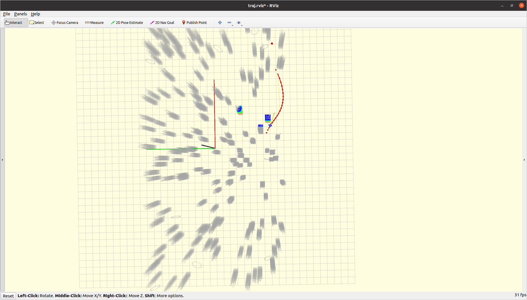
改变后:
cpp
dist_thresh = 20.0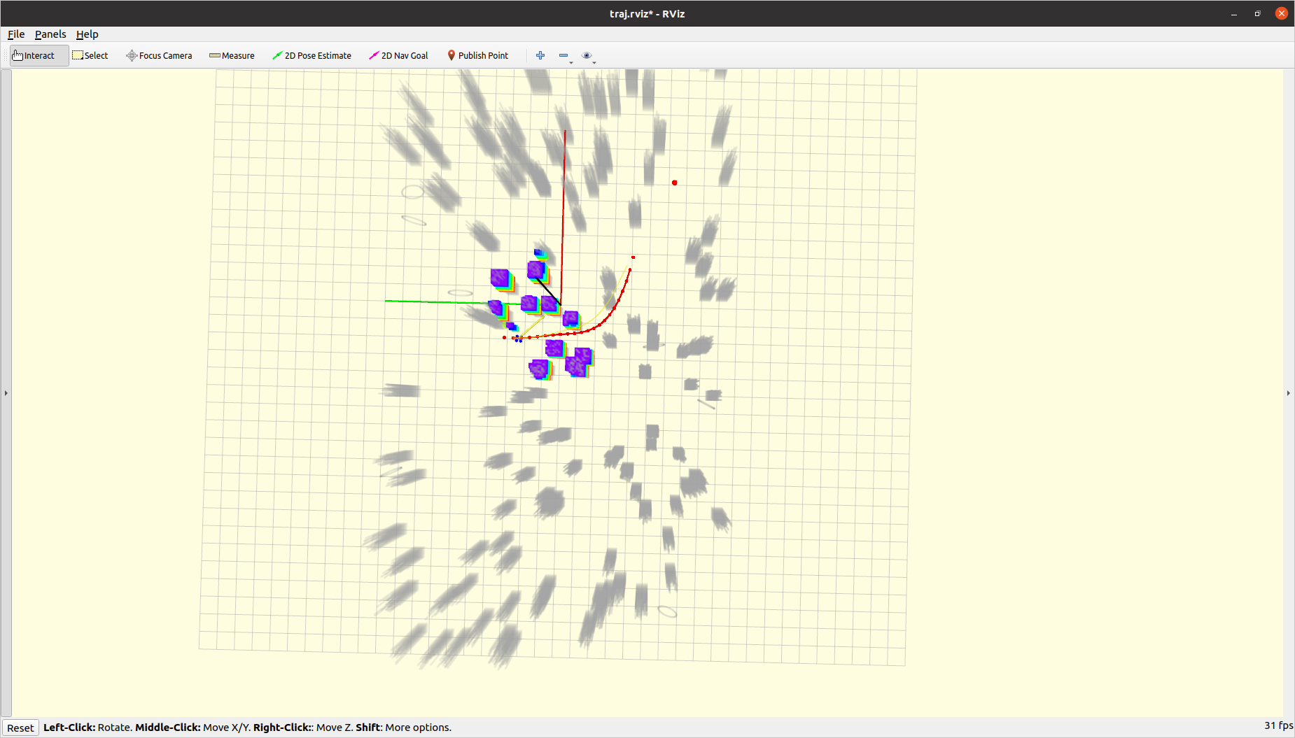 【注意】:运行之后发现并没有太大的区别。
最小化Sanp轨迹生成函数(核心实现)解读------函数minSnapTraj:
cpp
// 最小Snap轨迹生成函数(核心实现)
PolynomialTraj minSnapTraj(const Eigen::MatrixXd& Pos, const Eigen::Vector3d& start_vel,
                           const Eigen::Vector3d& end_vel, const Eigen::Vector3d& start_acc,
                           const Eigen::Vector3d& end_acc, const Eigen::VectorXd& Time) {

  // --- 初始化阶段 ---
  int seg_num = Time.size(); // 轨迹段数(航点间分段)
  Eigen::MatrixXd poly_coeff(seg_num, 3 * 6); // 存储XYZ三轴各6阶多项式系数
  Eigen::VectorXd Px(6 * seg_num), Py(6 * seg_num), Pz(6 * seg_num); // 各段多项式系数向量

  int num_f, num_p;  // number of fixed and free variables
  int num_d;         // number of all segments' derivatives

  // 阶乘计算lambda(用于导数项系数计算)
  const static auto Factorial = [](int x) {
    int fac = 1;
    for (int i = x; i > 0; i--)
      fac = fac * i;
    return fac;
  };

  /* ---------- end point derivative ---------- */
  // --- 端点导数约束设置 ---
  Eigen::VectorXd Dx = Eigen::VectorXd::Zero(seg_num * 6); // X轴各段导数约束
  Eigen::VectorXd Dy = Eigen::VectorXd::Zero(seg_num * 6);
  Eigen::VectorXd Dz = Eigen::VectorXd::Zero(seg_num * 6);

  for (int k = 0; k < seg_num; k++) {
    /* position to derivative */
    // 设置位置约束(每段起点和终点)
    Dx(k * 6) = Pos(k, 0);
    Dx(k * 6 + 1) = Pos(k + 1, 0);
    Dy(k * 6) = Pos(k, 1);
    Dy(k * 6 + 1) = Pos(k + 1, 1);
    Dz(k * 6) = Pos(k, 2);
    Dz(k * 6 + 1) = Pos(k + 1, 2);

    // 首段设置初始速度/加速度约束
    if (k == 0) {
      Dx(k * 6 + 2) = start_vel(0);
      Dy(k * 6 + 2) = start_vel(1);
      Dz(k * 6 + 2) = start_vel(2);

      Dx(k * 6 + 4) = start_acc(0);
      Dy(k * 6 + 4) = start_acc(1);
      Dz(k * 6 + 4) = start_acc(2);
    }
    // 末段设置终止速度/加速度约束
    else if (k == seg_num - 1) {
      Dx(k * 6 + 3) = end_vel(0);
      Dy(k * 6 + 3) = end_vel(1);
      Dz(k * 6 + 3) = end_vel(2);

      Dx(k * 6 + 5) = end_acc(0);
      Dy(k * 6 + 5) = end_acc(1);
      Dz(k * 6 + 5) = end_acc(2);
    }
  }

  /* ---------- Mapping Matrix A ---------- */
  // --- 构建映射矩阵A ---
  Eigen::MatrixXd Ab;
  Eigen::MatrixXd A = Eigen::MatrixXd::Zero(seg_num * 6, seg_num * 6);

  for (int k = 0; k < seg_num; k++) {
    Ab = Eigen::MatrixXd::Zero(6, 6);
    for (int i = 0; i < 3; i++) {
      Ab(2 * i, i) = Factorial(i);
      for (int j = i; j < 6; j++)
        Ab(2 * i + 1, j) = Factorial(j) / Factorial(j - i) * pow(Time(k), j - i);
    }
    A.block(k * 6, k * 6, 6, 6) = Ab;
  }

  /* ---------- Produce Selection Matrix C' ---------- */
  // --- 构建选择矩阵Ct ---
  Eigen::MatrixXd Ct, C;

  num_f = 2 * seg_num + 4;  // 3 + 3 + (seg_num - 1) * 2 = 2m + 4
  num_p = 2 * seg_num - 2;  //(seg_num - 1) * 2 = 2m - 2
  num_d = 6 * seg_num;
  Ct = Eigen::MatrixXd::Zero(num_d, num_f + num_p);
  Ct(0, 0) = 1;
  Ct(2, 1) = 1;
  Ct(4, 2) = 1;  // stack the start point
  Ct(1, 3) = 1;
  Ct(3, 2 * seg_num + 4) = 1;
  Ct(5, 2 * seg_num + 5) = 1;

  Ct(6 * (seg_num - 1) + 0, 2 * seg_num + 0) = 1;
  Ct(6 * (seg_num - 1) + 1, 2 * seg_num + 1) = 1;  // Stack the end point
  Ct(6 * (seg_num - 1) + 2, 4 * seg_num + 0) = 1;
  Ct(6 * (seg_num - 1) + 3, 2 * seg_num + 2) = 1;  // Stack the end point
  Ct(6 * (seg_num - 1) + 4, 4 * seg_num + 1) = 1;
  Ct(6 * (seg_num - 1) + 5, 2 * seg_num + 3) = 1;  // Stack the end point

  for (int j = 2; j < seg_num; j++) {
    Ct(6 * (j - 1) + 0, 2 + 2 * (j - 1) + 0) = 1;
    Ct(6 * (j - 1) + 1, 2 + 2 * (j - 1) + 1) = 1;
    Ct(6 * (j - 1) + 2, 2 * seg_num + 4 + 2 * (j - 2) + 0) = 1;
    Ct(6 * (j - 1) + 3, 2 * seg_num + 4 + 2 * (j - 1) + 0) = 1;
    Ct(6 * (j - 1) + 4, 2 * seg_num + 4 + 2 * (j - 2) + 1) = 1;
    Ct(6 * (j - 1) + 5, 2 * seg_num + 4 + 2 * (j - 1) + 1) = 1;
  }

  C = Ct.transpose();

  Eigen::VectorXd Dx1 = C * Dx;
  Eigen::VectorXd Dy1 = C * Dy;
  Eigen::VectorXd Dz1 = C * Dz;

  /* ---------- minimum snap matrix ---------- */
  // --- 构造最小Snap优化问题 ---
  Eigen::MatrixXd Q = Eigen::MatrixXd::Zero(seg_num * 6, seg_num * 6);
  // 计算Snap项积分(四阶导数平方的积分)
  for (int k = 0; k < seg_num; k++) {
    for (int i = 3; i < 6; i++) {
      for (int j = 3; j < 6; j++) {
        Q(k * 6 + i, k * 6 + j) =
            i * (i - 1) * (i - 2) * j * (j - 1) * (j - 2) / (i + j - 5) * pow(Time(k), (i + j - 5));
      }
    }
  }

  /* ---------- R matrix ---------- */
  // --- 求解闭式解 ---
  Eigen::MatrixXd R = C * A.transpose().inverse() * Q * A.inverse() * Ct;

  Eigen::VectorXd Dxf(2 * seg_num + 4), Dyf(2 * seg_num + 4), Dzf(2 * seg_num + 4);

  Dxf = Dx1.segment(0, 2 * seg_num + 4);
  Dyf = Dy1.segment(0, 2 * seg_num + 4);
  Dzf = Dz1.segment(0, 2 * seg_num + 4);

  Eigen::MatrixXd Rff(2 * seg_num + 4, 2 * seg_num + 4);
  Eigen::MatrixXd Rfp(2 * seg_num + 4, 2 * seg_num - 2);
  Eigen::MatrixXd Rpf(2 * seg_num - 2, 2 * seg_num + 4);
  Eigen::MatrixXd Rpp(2 * seg_num - 2, 2 * seg_num - 2);

  Rff = R.block(0, 0, 2 * seg_num + 4, 2 * seg_num + 4);
  Rfp = R.block(0, 2 * seg_num + 4, 2 * seg_num + 4, 2 * seg_num - 2);
  Rpf = R.block(2 * seg_num + 4, 0, 2 * seg_num - 2, 2 * seg_num + 4);
  Rpp = R.block(2 * seg_num + 4, 2 * seg_num + 4, 2 * seg_num - 2, 2 * seg_num - 2);

  /* ---------- close form solution ---------- */

  Eigen::VectorXd Dxp(2 * seg_num - 2), Dyp(2 * seg_num - 2), Dzp(2 * seg_num - 2);
  Dxp = -(Rpp.inverse() * Rfp.transpose()) * Dxf;
  Dyp = -(Rpp.inverse() * Rfp.transpose()) * Dyf;
  Dzp = -(Rpp.inverse() * Rfp.transpose()) * Dzf;

  Dx1.segment(2 * seg_num + 4, 2 * seg_num - 2) = Dxp;
  Dy1.segment(2 * seg_num + 4, 2 * seg_num - 2) = Dyp;
  Dz1.segment(2 * seg_num + 4, 2 * seg_num - 2) = Dzp;

  Px = (A.inverse() * Ct) * Dx1;
  Py = (A.inverse() * Ct) * Dy1;
  Pz = (A.inverse() * Ct) * Dz1;

  for (int i = 0; i < seg_num; i++) {
    poly_coeff.block(i, 0, 1, 6) = Px.segment(i * 6, 6).transpose();
    poly_coeff.block(i, 6, 1, 6) = Py.segment(i * 6, 6).transpose();
    poly_coeff.block(i, 12, 1, 6) = Pz.segment(i * 6, 6).transpose();
  }

  /* ---------- use polynomials ---------- */
  PolynomialTraj poly_traj;
  for (int i = 0; i < poly_coeff.rows(); ++i) {
    vector<double> cx(6), cy(6), cz(6);
    for (int j = 0; j < 6; ++j) {
      cx[j] = poly_coeff(i, j), cy[j] = poly_coeff(i, j + 6), cz[j] = poly_coeff(i, j + 12);
    }
    reverse(cx.begin(), cx.end());
    reverse(cy.begin(), cy.end());
    reverse(cz.begin(), cz.end());
    double ts = Time(i);
    poly_traj.addSegment(cx, cy, cz, ts);
  }

  return poly_traj;
}
函数定义和输入变量部分:
cpp
PolynomialTraj minSnapTraj(const Eigen::MatrixXd& Pos, const Eigen::Vector3d& start_vel,
                           const Eigen::Vector3d& end_vel, const Eigen::Vector3d& start_acc,
                           const Eigen::Vector3d& end_acc, const Eigen::VectorXd& Time) {
定义轨迹段数,定义进行拟合的多项式:
cpp
int seg_num = Time.size(); // 轨迹段数(航点间分段)
  Eigen::MatrixXd poly_coeff(seg_num, 3 * 6); // 存储XYZ三轴各6阶多项式系数
  Eigen::VectorXd Px(6 * seg_num), Py(6 * seg_num), Pz(6 * seg_num); // 各段多项式系数向量

  int num_f, num_p;  // number of fixed and free variables
  int num_d;         // number of all segments' derivatives
自定义计算x的阶乘函数:
cpp
// 阶乘计算lambda(用于导数项系数计算)
  const static auto Factorial = [](int x) {
    int fac = 1;
    for (int i = x; i > 0; i--)
      fac = fac * i;
    return fac;
  };
首末、以及各段的首末端点的硬约束:
cpp
// --- 端点导数约束设置 ---
  Eigen::VectorXd Dx = Eigen::VectorXd::Zero(seg_num * 6); // X轴各段导数约束
  Eigen::VectorXd Dy = Eigen::VectorXd::Zero(seg_num * 6);
  Eigen::VectorXd Dz = Eigen::VectorXd::Zero(seg_num * 6);

  for (int k = 0; k < seg_num; k++) {
    /* position to derivative */
    // 设置位置约束(每段起点和终点)
    Dx(k * 6) = Pos(k, 0);
    Dx(k * 6 + 1) = Pos(k + 1, 0);
    Dy(k * 6) = Pos(k, 1);
    Dy(k * 6 + 1) = Pos(k + 1, 1);
    Dz(k * 6) = Pos(k, 2);
    Dz(k * 6 + 1) = Pos(k + 1, 2);

    // 首段设置初始速度/加速度约束
    if (k == 0) {
      Dx(k * 6 + 2) = start_vel(0);
      Dy(k * 6 + 2) = start_vel(1);
      Dz(k * 6 + 2) = start_vel(2);

      Dx(k * 6 + 4) = start_acc(0);
      Dy(k * 6 + 4) = start_acc(1);
      Dz(k * 6 + 4) = start_acc(2);
    }
    // 末段设置终止速度/加速度约束
    else if (k == seg_num - 1) {
      Dx(k * 6 + 3) = end_vel(0);
      Dy(k * 6 + 3) = end_vel(1);
      Dz(k * 6 + 3) = end_vel(2);

      Dx(k * 6 + 5) = end_acc(0);
      Dy(k * 6 + 5) = end_acc(1);
      Dz(k * 6 + 5) = end_acc(2);
    }
  }
构建A矩阵:
cpp
// --- 构建映射矩阵A ---
  Eigen::MatrixXd Ab;
  Eigen::MatrixXd A = Eigen::MatrixXd::Zero(seg_num * 6, seg_num * 6);

  for (int k = 0; k < seg_num; k++) {
    Ab = Eigen::MatrixXd::Zero(6, 6);
    for (int i = 0; i < 3; i++) {
      Ab(2 * i, i) = Factorial(i);
      for (int j = i; j < 6; j++)
        Ab(2 * i + 1, j) = Factorial(j) / Factorial(j - i) * pow(Time(k), j - i);
    }
    A.block(k * 6, k * 6, 6, 6) = Ab;
}【注意】:A矩阵的构建与阶数有关,跟时间Time有关,它是由于微分约束的原因,但是我们并没有限制轨迹必须通过某一些点,或者以一个确定的状态通过某一些中间的航迹点。也就是上述的这些多项式系数中,有一些是已知的。但是大多数情况下,我们都是对轨迹的位置有一些限制的,并不能随意生成,所以还需要给中间的航迹点加一些限制。包括位置、速度、加速度、Jerk、Snap等等的限制。
可以参考博客:【附源码和详细的公式推导】Minimum Snap轨迹生成,闭式求解Minimum Snap问题,机器人轨迹优化,多项式轨迹路径生成与优化-CSDN博客
构建C矩阵:
cpp
// --- 构建选择矩阵Ct ---
  Eigen::MatrixXd Ct, C;

  num_f = 2 * seg_num + 4;  // 3 + 3 + (seg_num - 1) * 2 = 2m + 4
  num_p = 2 * seg_num - 2;  //(seg_num - 1) * 2 = 2m - 2
  num_d = 6 * seg_num;
  Ct = Eigen::MatrixXd::Zero(num_d, num_f + num_p);
// 固定约束部分(起点终点位置速度加速度)
  Ct(0, 0) = 1;
  Ct(2, 1) = 1;
  Ct(4, 2) = 1;  // stack the start point
  Ct(1, 3) = 1;
  Ct(3, 2 * seg_num + 4) = 1;
  Ct(5, 2 * seg_num + 5) = 1;

  Ct(6 * (seg_num - 1) + 0, 2 * seg_num + 0) = 1;
  Ct(6 * (seg_num - 1) + 1, 2 * seg_num + 1) = 1;  // Stack the end point
  Ct(6 * (seg_num - 1) + 2, 4 * seg_num + 0) = 1;
  Ct(6 * (seg_num - 1) + 3, 2 * seg_num + 2) = 1;  // Stack the end point
  Ct(6 * (seg_num - 1) + 4, 4 * seg_num + 1) = 1;
  Ct(6 * (seg_num - 1) + 5, 2 * seg_num + 3) = 1;  // Stack the end point
// ...(中间段连续性约束填充)

  for (int j = 2; j < seg_num; j++) {
    Ct(6 * (j - 1) + 0, 2 + 2 * (j - 1) + 0) = 1;
    Ct(6 * (j - 1) + 1, 2 + 2 * (j - 1) + 1) = 1;
    Ct(6 * (j - 1) + 2, 2 * seg_num + 4 + 2 * (j - 2) + 0) = 1;
    Ct(6 * (j - 1) + 3, 2 * seg_num + 4 + 2 * (j - 1) + 0) = 1;
    Ct(6 * (j - 1) + 4, 2 * seg_num + 4 + 2 * (j - 2) + 1) = 1;
    Ct(6 * (j - 1) + 5, 2 * seg_num + 4 + 2 * (j - 1) + 1) = 1;
  }

  C = Ct.transpose();

  Eigen::VectorXd Dx1 = C * Dx;
  Eigen::VectorXd Dy1 = C * Dy;
Eigen::VectorXd Dz1 = C * Dz;【注意】:C矩阵是希望在A矩阵的基础上,加入连续性约束,使得微分约束和连续性约束成为一个整体,它是由于每一段轨迹与下一段轨迹需要连续性约束,也就是导数需要限制中间的航迹点在两段轨迹的接合处是左右两边状态要连续。如果我们要最小化的目标是Jerk,那么我们必须保证接合处三阶导数是连续的。
构建最小Snap优化问题,即QP问题:
cpp
// --- 构造最小Snap优化问题 ---
  Eigen::MatrixXd Q = Eigen::MatrixXd::Zero(seg_num * 6, seg_num * 6);
  // 计算Snap项积分(四阶导数平方的积分)
  for (int k = 0; k < seg_num; k++) {
    for (int i = 3; i < 6; i++) {
      for (int j = 3; j < 6; j++) {
        Q(k * 6 + i, k * 6 + j) =
            i * (i - 1) * (i - 2) * j * (j - 1) * (j - 2) / (i + j - 5) * pow(Time(k), (i + j - 5));
      }
    }
}【注意】:也就是QP问题,Q矩阵只与时间Time有关,其余的就是跟多项式系数有一定的关系。
闭式求解:
cpp
// --- 求解闭式解 ---
  Eigen::MatrixXd R = C * A.transpose().inverse() * Q * A.inverse() * Ct;

  Eigen::VectorXd Dxf(2 * seg_num + 4), Dyf(2 * seg_num + 4), Dzf(2 * seg_num + 4);

  Dxf = Dx1.segment(0, 2 * seg_num + 4);
  Dyf = Dy1.segment(0, 2 * seg_num + 4);
  Dzf = Dz1.segment(0, 2 * seg_num + 4);

  Eigen::MatrixXd Rff(2 * seg_num + 4, 2 * seg_num + 4);
  Eigen::MatrixXd Rfp(2 * seg_num + 4, 2 * seg_num - 2);
  Eigen::MatrixXd Rpf(2 * seg_num - 2, 2 * seg_num + 4);
  Eigen::MatrixXd Rpp(2 * seg_num - 2, 2 * seg_num - 2);

  Rff = R.block(0, 0, 2 * seg_num + 4, 2 * seg_num + 4);
  Rfp = R.block(0, 2 * seg_num + 4, 2 * seg_num + 4, 2 * seg_num - 2);
  Rpf = R.block(2 * seg_num + 4, 0, 2 * seg_num - 2, 2 * seg_num + 4);
  Rpp = R.block(2 * seg_num + 4, 2 * seg_num + 4, 2 * seg_num - 2, 2 * seg_num - 2);

  /* ---------- close form solution ---------- */

  Eigen::VectorXd Dxp(2 * seg_num - 2), Dyp(2 * seg_num - 2), Dzp(2 * seg_num - 2);
  Dxp = -(Rpp.inverse() * Rfp.transpose()) * Dxf;
  Dyp = -(Rpp.inverse() * Rfp.transpose()) * Dyf;
  Dzp = -(Rpp.inverse() * Rfp.transpose()) * Dzf;

  Dx1.segment(2 * seg_num + 4, 2 * seg_num - 2) = Dxp;
  Dy1.segment(2 * seg_num + 4, 2 * seg_num - 2) = Dyp;
Dz1.segment(2 * seg_num + 4, 2 * seg_num - 2) = Dzp;【注意】:根据QP问题,和数学性质,可以通过转化为无约束的最优化问题进行求解,就叫闭式求解。
重新构建多项式系数:
cpp
Px = (A.inverse() * Ct) * Dx1;
  Py = (A.inverse() * Ct) * Dy1;
  Pz = (A.inverse() * Ct) * Dz1;

  for (int i = 0; i < seg_num; i++) {
    poly_coeff.block(i, 0, 1, 6) = Px.segment(i * 6, 6).transpose();
    poly_coeff.block(i, 6, 1, 6) = Py.segment(i * 6, 6).transpose();
    poly_coeff.block(i, 12, 1, 6) = Pz.segment(i * 6, 6).transpose();
  }
重新构建轨迹对象:
cpp
/* ---------- use polynomials ---------- */
  PolynomialTraj poly_traj;
  for (int i = 0; i < poly_coeff.rows(); ++i) {
    vector<double> cx(6), cy(6), cz(6);
    for (int j = 0; j < 6; ++j) {
      cx[j] = poly_coeff(i, j), cy[j] = poly_coeff(i, j + 6), cz[j] = poly_coeff(i, j + 12);
    }
    reverse(cx.begin(), cx.end());
    reverse(cy.begin(), cy.end());
    reverse(cz.begin(), cz.end());
    double ts = Time(i);
    poly_traj.addSegment(cx, cy, cz, ts);
  }

  return poly_traj;
}
以上为fast-planner中Minum-snap的解析,代码为C++版本的,为了更好的进行迁移,接下来介绍python版本的Minnum-snap库算法。
python中的Minsnap轨迹规划代码库
官网:minsnap-trajectories · PyPI
类似于differential flatness, minimum snap, path planning, trajectory generation相关的轨迹生成python代码其中均可以实现。
由于上述代码库不好使用,遂找到了开源的手搓的三维Minsnap相关python代码,并进行了整理:
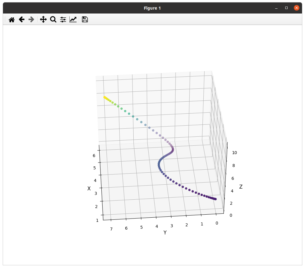
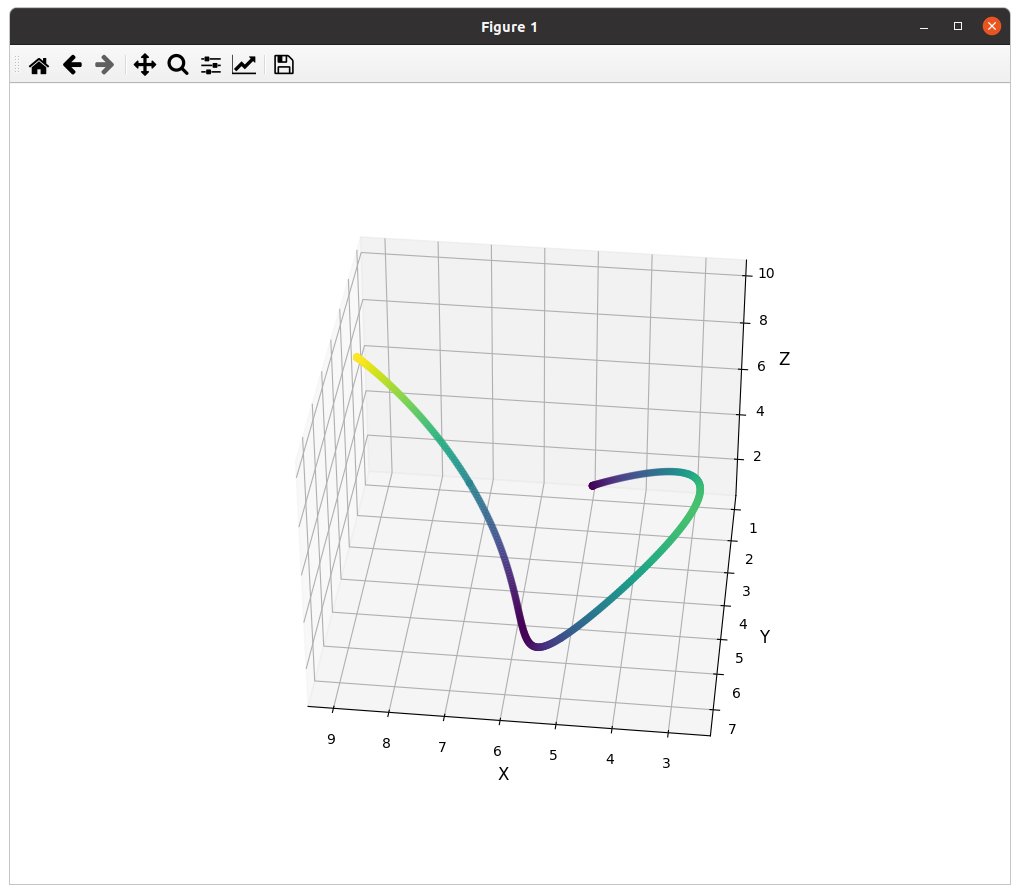
最小化Snap的结果:
python
# -*- coding: utf-8 -*-
import numpy as np
import matplotlib.pyplot as plt
from cvxopt import matrix, solvers
import open3d as o3d
from scipy.interpolate import splprep, splev,splder
import gurobipy as gp

class TrajectoryPlanner:
    _instance = None

    def __new__(cls):
        if cls._instance is None:
            cls._instance = super(TrajectoryPlanner, cls).__new__(cls)
            cls._instance.__initialized = False
        return cls._instance

    def __init__(self):
        if self.__initialized:
            return
        self.__initialized = True

        # 设置numpy打印参数:完全显示数组/禁止科学计数法/每行显示100字符
        np.set_printoptions(threshold=np.inf, suppress=True, linewidth=100)

        # 新增全局约束参数(单位:m/s, m/s²)
        self.MAX_VEL = 2.0  # 最大速度
        self.MIN_VEL = -2.0  # 最小速度(允许倒车时设为负值)
        self.MAX_ACC = 2.0  # 最大加速度
        self.MIN_ACC = -2.0  # 最小加速度(制动限制)
        self.deltaT = 0.5 #默认时间间隔
    def farthest_point_sampling(self,points, n_samples):
        indices = np.zeros(n_samples, dtype=int)
        distances = np.full(points.shape[0], np.inf)
        start_idx = np.random.randint(len(points))

        for i in range(n_samples):
            indices[i] = start_idx
            dist = np.linalg.norm(points - points[start_idx], axis=1)
            distances = np.minimum(distances, dist)
            start_idx = np.argmax(distances)

        return points[indices]

    def build_velocity_constraint_row(self, k, t, N):
        row = np.zeros(N)
        coeff = [0, 1, 2*t, 3*t**2, 4*t**3, 5*t**4, 6*t**5, 7*t**6]
        row[k*8 : (k+1)*8] = coeff
        return row

    def build_acceleration_constraint_row(self, k, t, N):
        row = np.zeros(N)
        coeff = [0, 0, 2, 6*t, 12*t**2, 20*t**3, 30*t**4, 0]  # 修正二阶导数项[3]
        row[k*8 : (k+1)*8] = coeff
        return row
    def getpos(self, x, v_start):
        """生成轨迹的最小加加速度(snap)优化路径

        参数:
            x : 路径点某一维度的坐标序列

        返回:
            Pos, Vel, Acc, Jer : 位置、速度、加速度、加加速度轨迹
        """
        self.deltaT = 0.2
        print(self.deltaT)
        T = np.linspace(0, self.deltaT * (len(x) - 1), len(x))  # 时间节点生成

        # 轨迹参数设置
        K = 4  # 最小化加加加速度(snap)对应四阶导数
        n_order = 2 * K - 1  # 多项式阶数(7次多项式)
        M = int(len(x)) - 1  # 轨迹分段数(路径点数量-1)
        N = M * (n_order + 1)  # 优化变量总维度(每段8个系数)

        def getQk(T_down, T_up):
            Q = np.zeros((8, 8))
            T_up2 = T_up**2
            T_up3 = T_up**3
            T_up4 = T_up**4
            T_up5 = T_up**5
            T_up6 = T_up**6
            T_up7 = T_up**7
            T_down2 = T_down**2
            T_down3 = T_down**3
            T_down4 = T_down**4
            T_down5 = T_down**5
            T_down6 = T_down**6
            T_down7 = T_down**7

            Q[4][5] = 1440 * (T_up2 - T_down2)
            Q[4][6] = 2880 * (T_up3 - T_down3)
            Q[4][7] = 5040 * (T_up4 - T_down4)
            Q[5][6] = 10800 * (T_up4 - T_down4)
            Q[5][7] = 20160 * (T_up5 - T_down5)
            Q[6][7] = 50400 * (T_up6 - T_down6)
            Q = Q + Q.T

            Q[4][4] = 576 * (T_up - T_down)
            Q[5][5] = 4800 * (T_up3 - T_down3)
            Q[6][6] = 25920 * (T_up5 - T_down5)
            Q[7][7] = 100800 * (T_up7 - T_down7)
            return Q

        # 构造全局Q矩阵(块对角矩阵)
        Q = np.zeros((N, N))
        for k in range(1, M + 1):  # 遍历每个轨迹段
            Qk = getQk(T[k - 1], T[k])
            # 块填充策略:每段8x8的Qk矩阵放在对角线位置
            Q[(8*(k-1)) : (8*k), (8*(k-1)) : (8*k)] = Qk
        Q = Q * 2  # 二次规划标准形式需要乘以1/2,这里提前补偿

        # 构造等式约束矩阵A
        A0 = np.zeros((2*K + M - 1, N))  # 起点/终点约束 + 中间点约束
        b0 = np.zeros(len(A0))

        # 起点/终点的位置、速度、加速度、加加速度约束
        for k in range(K):  # 0-3阶导数约束
            for i in range(k, 8):  # 多项式系数遍历
                c = 1
                for j in range(k):
                    c *= (i - j)  # 导数系数计算
                # 起点速度约束(k=1时)
                if k == 1:
                    A0[2][i] = c * T[0]**(i - k)  # 起点速度行索引2
                    # 填充速度约束值到b0
                    b0[2] = v_start  # 起始速度预设值
                # 起点约束(t=0时各阶导数)
                A0[0 + k*2][i] = c * T[0]**(i - k)
                # 终点约束(t=T时各阶导数)
                A0[1 + k*2][(M-1)*8 + i] = c * T[M]**(i - k)
        b0[0] = x[0]  # 起点位置约束值
        b0[1] = x[M]  # 终点位置约束值

        # 中间点位置约束
        for m in range(1, M):
            for i in range(8):
                A0[8 + m-1][m*8 + i] = T[m]**i  # 时间多项式基函数
            b0[8 + m-1] = x[m]  # 中间点位置约束值

        # 轨迹段连接处的连续性约束(位置-加加速度连续)
        A1 = np.zeros(((M-1)*K, N))
        b1 = np.zeros(len(A1))
        for m in range(M-1):  # 遍历每个连接点
            for k in range(K):  # 0-3阶导数连续
                for i in range(k, 8):  # 多项式系数
                    c = 1
                    for j in range(k):
                        c *= (i - j)  # 导数系数乘积
                    index = m*4 + k
                    # 前一段轨迹末状态
                    A1[index][m*8 + i] = c * T[m+1]**(i - k)
                    # 后一段轨迹初状态(符号取反)
                    A1[index][(m+1)*8 + i] = -c * T[m+1]**(i - k)

        # 合并所有约束条件
        A = np.vstack((A0, A1))
        b = np.hstack((b0, b1))

        # 转换为cvxopt需要的矩阵格式
        Q_mat = matrix(Q)
        q_mat = matrix(np.zeros(N))
        A_mat = matrix(A)
        b_mat = matrix(b)

        # 求解二次规划问题(网页7提到的凸优化方法)
        # result = solvers.qp(Q_mat, q_mat, A=A_mat, b=b_mat)
        # ============ 求解器调用改造 ============
        result = solvers.qp(Q_mat, q_mat, A=A_mat, b=b_mat)
        p_coff = np.asarray(result['x']).flatten()  # 获取多项式系数

        # 轨迹重构与导数计算
        Pos = []; Vel = []; Acc = []; Jer = []
        for k in range(M):  # 遍历每个轨迹段
            t = np.linspace(T[k], T[k + 1], 100)
            t_pos = np.vstack((t**0, t**1, t**2, t**3, t**4, t**5, t**6, t**7))
            t_vel = np.vstack((t*0, t**0, 2 * t**1, 3 * t**2, 4 * t**3, 5 * t**4, 6*t**5, 7*t**6))
            t_acc = np.vstack((t*0, t*0, 2 * t**0, 3 * 2 * t**1, 4 * 3 * t**2, 5 * 4 * t**3, 6*5*t**4, 7*6*t**5))
            t_jer = np.vstack((t*0, t*0, t*0, 3 * 2 * t**0, 4 * 3 *2* t**1, 5 * 4 *3* t**2, 6*5*4*t**3, 7*6*5*t**4))
            coef = p_coff[k * 8 : (k + 1) * 8]
            coef = np.reshape(coef, (1, 8))
            pos = coef.dot(t_pos)
            vel = coef.dot(t_vel)
            acc = coef.dot(t_acc)
            jer = coef.dot(t_jer)
            Pos.append([t, pos[0]])
            Vel.append([t, vel[0]])
            Acc.append([t, acc[0]])
            Jer.append([t, jer[0]])

        return np.array(Pos), np.array(Vel), np.array(Acc), np.array(Jer)

    def merge_axis_data(self, data):
        """合并三维轨迹数据为连续时间序列"""
        time = np.concatenate(data[:, 0, :].T)  # 时间轴
        values = np.concatenate(data[:, 1, :].T)  # 数值轴
        return time, values
    def smooth_3d_path(self,path, s=1.0):
        """三维路径B样条平滑"""
        path = np.array(path)
        if len(path) < 10:  # 样条需要至少4个点
            return path
        tck, u = splprep(path.T, s=s)
        if len(path) > 10:
            num_len = int(len(path)/2)
        else:
            num_len = int(len(path))
        new_points = splev(np.linspace(0,1,num_len), tck)

        return np.column_stack(new_points)

    def plot_trajectory(self, path, initial_vel, plot_flag=True):
        path = np.array(path)  # 转换为numpy数组
        initial_vel = np.array(initial_vel)
        displacements = np.diff(path, axis=0)  # 形状:(N-1, 3) 的位移向量
        distances = np.linalg.norm(displacements, axis=1)  # 沿轴1计算每个向量的范数
        self.deltaT = np.max(distances) / self.MAX_VEL
        print(self.deltaT)
        # 分别处理三个维度的轨迹
        Posx, Velx, Accx, Jerx = self.getpos(path[:, 0], initial_vel[0])  # X轴轨迹
        Posy, Vely, Accy, Jery = self.getpos(path[:, 1], initial_vel[1])  # Y轴轨迹
        Posz, Velz, Accz, Jerz = self.getpos(path[:, 2], initial_vel[2])  # Z轴轨迹

        # 合并所有轨迹点的三维坐标
        x = np.concatenate(Posx[:, 1, :].T)  # X坐标序列
        y = np.concatenate(Posy[:, 1, :].T)  # Y坐标序列
        z = np.concatenate(Posz[:, 1, :].T)  # Z坐标序列

        # 将三维坐标组合成一个优化路径
        optimization_path = np.column_stack((x, y, z))
        # 如果plot_flag为True,则绘制三维轨迹图
        if plot_flag:
            # 三维轨迹可视化
            fig = plt.figure(figsize=(10, 8))
            ax = fig.add_subplot(111, projection='3d')

            # 绘制三维散点图
            ax.scatter3D(x[::5], y[::5], z[::5],
                        c=z[::5],  # 颜色映射Z值
                        cmap='viridis',  # 使用viridis色图
                        s=20)  # 点的大小

            # 设置坐标轴标签和观察视角
            ax.set_xlabel('X', fontsize=12)
            ax.set_ylabel('Y', fontsize=12)
            ax.set_zlabel('Z', fontsize=12)
            ax.view_init(elev=30, azim=45)  # 仰角30度,方位角45度

            # 绘制速度图
            time_x, vel_x = self.merge_axis_data(Velx)
            time_y, vel_y = self.merge_axis_data(Vely)
            time_z, vel_z = self.merge_axis_data(Velz)

            plt.figure(figsize=(12, 6))
            plt.scatter(time_x, vel_x, color='red', s=10, label='X', marker='o')  # X轴速度点
            plt.scatter(time_y, vel_y, color='green', s=10, label='Y', marker='s')  # Y轴速度点
            plt.scatter(time_z, vel_z, color='blue', s=10, label='Z', marker='^')  # Z轴速度点

            # 美化设置
            plt.xlabel('time (s)', fontsize=12)
            plt.ylabel('vel (m/s)', fontsize=12)
            plt.title('vel', fontsize=14)
            plt.grid(True, linestyle='--', alpha=0.5)
            plt.legend(loc='upper right', frameon=False)
            plt.tight_layout()

            # 绘制加速度图
            time_x, acc_x = self.merge_axis_data(Accx)
            time_y, acc_y = self.merge_axis_data(Accy)
            time_z, acc_z = self.merge_axis_data(Accz)

            plt.figure(figsize=(12, 6))
            plt.scatter(time_x, acc_x, color='#FF6347', s=10, label='X', marker='o')  # 番茄红
            plt.scatter(time_y, acc_y, color='#20B2AA', s=10, label='Y', marker='o')  # 浅海绿
            plt.scatter(time_z, acc_z, color='#6A5ACD', s=10, label='Z', marker='o')  # 板岩蓝

            # 美化设置
            plt.xlabel('time (s)', fontsize=12)
            plt.ylabel('a (m/(s**2))', fontsize=12)
            plt.title('a', fontsize=14)
            plt.grid(True, linestyle='--', alpha=0.5)
            plt.legend(loc='upper right', frameon=False)
            plt.tight_layout()

            # 绘制加加速度图
            time_x, jerx = self.merge_axis_data(Jerx)
            time_y, jery = self.merge_axis_data(Jery)
            time_z, jerz = self.merge_axis_data(Jerz)

            plt.figure(figsize=(12, 6))
            plt.scatter(time_x, jerx, color='#FF6347', s=10, label='X', marker='o')  # 番茄红
            plt.scatter(time_y, jery, color='#20B2AA', s=10, label='Y', marker='o')  # 浅海绿
            plt.scatter(time_z, jerz, color='#6A5ACD', s=10, label='Z', marker='o')  # 板岩蓝

            # 美化设置
            plt.xlabel('time (s)', fontsize=12)
            plt.ylabel('jerk (m/(s**3))', fontsize=12)
            plt.title('jerk', fontsize=14)
            plt.grid(True, linestyle='--', alpha=0.5)
            plt.legend(loc='upper right', frameon=False)
            plt.tight_layout()

            # 显示所有图像
            plt.show()

        # 返回优化路径
        return optimization_path


if __name__ == "__main__":
    # planner = TrajectoryPlanner()
    path = [[1, 1, 1], [2, 2, 1], [3, 3, 2], [4, 4, 3], [5, 5, 10]]
    initial_vel = [0.5, 0.5, 0.5]

    # 绘图并返回优化路径
    optimization_path = TrajectoryPlanner().plot_trajectory(path, initial_vel, plot_flag=False)
    print("Optimization Path:\n", optimization_path)