目录
- [1 控制采样 vs 状态采样](#1 控制采样 vs 状态采样)
- [2 State Lattice路径规划](#2 State Lattice路径规划)
-
- [2.1 算法流程](#2.1 算法流程)
- [2.2 Lattice运动基元生成](#2.2 Lattice运动基元生成)
- [2.3 几何代价函数](#2.3 几何代价函数)
- [2.4 运动学约束启发式](#2.4 运动学约束启发式)
- [3 算法仿真](#3 算法仿真)
-
- [3.1 ROS C++仿真](#3.1 ROS C++仿真)
- [3.2 Python仿真](#3.2 Python仿真)
1 控制采样 vs 状态采样
控制采样的技术路线源自经典的运动学建模思想。这种方法将机器人的控制指令空间进行离散化,预设一组基础运动模式(如固定转向角、恒定速度等),通过前向积分生成候选路径。以差速驱动机器人为例,算法可能预设
- 左转30度
- 直行
- 右转30度
三种基础控制指令,在规划时将这些指令按不同时长组合,形成扇形展开的候选路径集,如下图(a)所示。这种方法的优势在于物理可解释性强,易于求解。但其局限性同样显著:当环境障碍复杂时,由于缺乏目标导向,规划效率较低
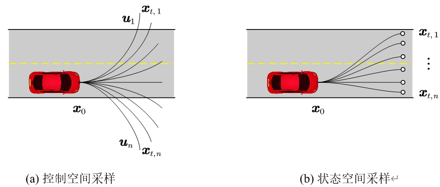
状态采样则直接在目标状态空间(如位置、朝向)中离散化采样点,通过最优控制或数值优化反向求解连接当前状态与目标状态的可行轨迹,如上图(b)所示。例如在自动驾驶场景中,算法可能在车辆前方50米处均匀采样多个目标位姿,再通过多项式曲线或回旋曲线连接起点与终点。这种方法的优势在于解空间覆盖度高,能够生成形态多样的候选路径,特别适合结构化道路中需要精确贴合车道线的场景。但代价是计算复杂度显著增加,反向轨迹求解可能涉及大量迭代优化,实时性面临挑战。
两种方法在工程实践中的博弈,折射出路径规划领域的核心矛盾------解空间完备性与计算效率的平衡。本节介绍的状态晶格State Lattice路径规划就属于状态空间采样类的方法,下面详细阐述
2 State Lattice路径规划
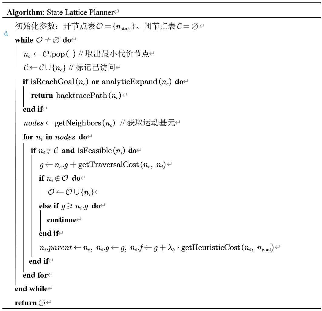
2.1 算法流程
先宏观地展示算法流程
其中的核心概念总结如下:
- 状态晶格(State Lattice) 将机器人的状态空间(位置、方向等)离散化为一系列相连的状态点,形成网格状结构
- 开节点表(Open List) 存储待评估探索的节点集合,按照代价排序
- 闭节点表(Closed List) 存储已经评估处理过的节点集合
- 节点(Node) 表示状态空间中的一个点,包含位置、方向、代价等信息
- 运动基元(Motion Primitive) 预定义的合法移动方式,确保路径满足动力学约束
可以看到,State Lattice同样遵守A*算法框架,可以对比:
- 路径规划 | 图解A*、Dijkstra、GBFS算法的异同(附C++/Python/Matlab仿真)
- 路径规划 | 详解混合A*算法Hybrid A*(附ROS C++/Python/Matlab仿真)
不同在于,State Lattice规划器在状态空间采样一系列节点生成运动基元,而A*或混合A*算法则是在控制空间采样。那么,状态空间运动基元是如何生成的呢?
2.2 Lattice运动基元生成
设机器人状态空间为
s = x , y , θ T s=x,y,\\theta^T s=x,y,θT
如下图所示,机器人用绿色矩形框表示,在圆周上等距离地采样一系列点作为状态采样点 x i , y i , θ i x_i,y_i, \\theta_i xi,yi,θi,问题转变为已知起始状态 x 0 , y 0 , θ 0 x_0,y_0,\\theta_0 x0,y0,θ0和各个终止状态 x i , y i , θ i x_i,y_i, \\theta_i xi,yi,θi,如何生成一条连接两个状态的运动学可行路径的问题,即如何生成下图所示的蓝色与红色路径
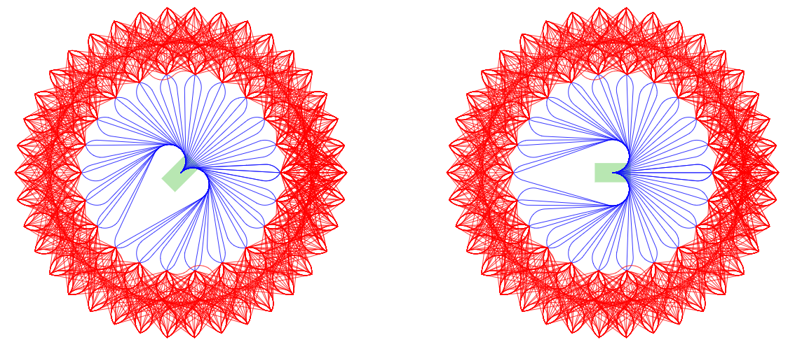
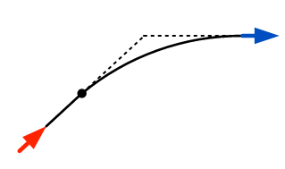
求解的方法有很多,例如转化为两点边值问题、最优控制优化问题等,但为了简明起见,本节介绍一种解析几何的方法。如下图所示,设首末方向向量交点为 P P P,首末端点分别为 A A A、 B B B,不失一般性假定 ∣ P A ∣ ≥ ∣ P B ∣ |PA|≥|PB| ∣PA∣≥∣PB∣,则在线段 P A PA PA上从 P P P出发截取 ∣ P B ∣ |PB| ∣PB∣长度的子线段 P C PC PC,以 B B B和 C C C为两个端点构造圆弧,产生由 A C AC AC和 C B ⏠ \overgroup{CB} CB 组成的单线段单圆弧轨迹;特别地,当 ∣ P A ∣ = ∣ P B ∣ \left| PA \right|=\left| PB \right| ∣PA∣=∣PB∣时 ∣ A C ∣ = 0 \left| AC \right|=0 ∣AC∣=0,退化为单圆弧轨迹
2.3 几何代价函数
基于上述几何关系可以定义基本代价函数
C a d j u s t = { C b a s e i f 直线运动 C b a s e ⋅ P n o n s t r a i g h t i f 同向转弯 C b a s e ⋅ ( P n o n s t r a i g h t + P c h a n g e ) i f 转向切换 C_{\mathrm{adjust}}=\begin{cases} C_{\mathrm{base}}\,\,& \mathrm{if} \text{直线运动}\\ C_{\mathrm{base}}\cdot P_{\mathrm{nonstraight}}& \mathrm{if} \text{同向转弯}\\ C_{\mathrm{base}}\cdot \left( P_{\mathrm{nonstraight}}+P_{\mathrm{change}} \right)& \mathrm{if} \text{转向切换}\\\end{cases} Cadjust=⎩ ⎨ ⎧CbaseCbase⋅PnonstraightCbase⋅(Pnonstraight+Pchange)if直线运动if同向转弯if转向切换
其中 C b a s e = L p r i m ⋅ P t r a v e l C_{\mathrm{base}}=L_{\mathrm{prim}}\cdot P_{\mathrm{travel}} Cbase=Lprim⋅Ptravel, L p r i m L_{\mathrm{prim}} Lprim是运动基元路径长度。为了考虑纯转向和反向运动,进一步修正代价函数为
C = { P r o t a t e i f L p r i m < ϵ C a d j u s t ⋅ P r e v e r s e i f 反向运动 C a d j u s t o t h e r w i s e C=\begin{cases} P_{\mathrm{rotate}}\,\,& \mathrm{if} L_{\mathrm{prim}}<\epsilon\\ C_{\mathrm{adjust}}\cdot P_{\mathrm{reverse}}& \mathrm{if} \text{反向运动}\\ C_{\mathrm{adjust}}& \mathrm{otherwise}\\\end{cases} C=⎩ ⎨ ⎧ProtateCadjust⋅PreverseCadjustifLprim<ϵif反向运动otherwise
2.4 运动学约束启发式
A*算法的启发式函数一般采用当前点到目标点的欧氏距离,State Lattice算法则向启发式函数进一步引入运动学约束
h ( n ) = max { C o n s t r a i n e d C o s t , U n c o n s t r a i n e d C o s t } h\left( n \right) =\max \left\{ \mathrm{ConstrainedCost},\mathrm{UnconstrainedCost} \right\} h(n)=max{ConstrainedCost,UnconstrainedCost}
其中:
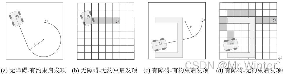
- C o n s t r a i n e d C o s t \mathrm{ConstrainedCost} ConstrainedCost:只考虑车辆的非完整运动学约束而不考虑障碍物的有约束启发项(Constrained heuristics),通常采用Dubins或Reeds-Shepp曲线计算该项损失。
- Dubins曲线 是指由美国数学家 Lester Dubins 在20世纪50年代提出的一种特殊类型的最短路径曲线。这种曲线通常用于描述在给定转弯半径下的无人机、汽车或船只等载具的最短路径,其特点是起始点和终点处的切线方向和曲率都是已知的,Dubins曲线包括直线段和最大转弯半径下的圆弧组成,通过合适的组合可以实现从一个姿态到另一个姿态的最短路径规划。更详细的算法原理请看曲线生成 | 图解Dubins曲线生成原理(附ROS C++/Python/Matlab仿真);
- Reeds-Shepp曲线 是一种用于描述在平面上从一个点到另一个点最优路径的数学模型。这种曲线是由美国数学家 J. A. Reeds 和 L. A. Shepp 在1990年提出的,它被广泛应用于路径规划和运动规划问题中,具有最优性、约束性和多样性,更详细的算法原理请看曲线生成 | 图解Reeds-Shepp曲线生成原理(附ROS C++/Python/Matlab仿真);
- 只考虑障碍物信息而不考虑车辆运动学特性的无约束启发项(Unconstrained heuristics),通常采用Dijkstra或A*算法计算该项损失。
如图所示,可视化了不同类型的启发项。当环境障碍不影响规划路径时,有约束启发项损失往往大于无约束,因为后者没有考虑朝向和运动限制;当环境障碍影响规划路径时,有约束启发项损失往往小于无约束,因为后者会进行避障。因此对两项取 max \max max算子可以综合障碍影响和运动学特性,更符合真实情况。
3 算法仿真
3.1 ROS C++仿真
核心代码如下所示
cpp
bool StateLatticePathPlanner::createPath(const Point3d& start, const Point3d& goal, Points3d& path, Points3d& expand)
{
  clearGraph();
  clearQueue();
  auto start_node = addToGraph(getIndex(start));
  auto goal_node = addToGraph(getIndex(goal));

  precomputeObstacleHeuristic(goal_node);

  // 0) Add starting point to the open set
  addToQueue(0.0, start_node);
  start_node->setAccumulatedCost(0.0);
  std::vector<NodeLattice::NodePtr> neighbors;  // neighbors of current node
  NodeLattice::NodePtr neighbor = nullptr;

  // main loop
  int iterations = 0, approach_iterations = 0;
  while (iterations < search_info_.max_iterations && !queue_.empty())
  {
    // 1) Pick the best node (Nbest) from open list
    NodeLattice::NodePtr current_node = queue_.top().second;
    queue_.pop();

    // Save current node coordinates for debug
    expand.emplace_back(current_node->pose().x(), current_node->pose().y(),
                        motion_table_.getAngleFromBin(current_node->pose().theta()));

    // Current node exists in closed list
    if (current_node->is_visited())
    {
      continue;
    }
    iterations++;

    // 2) Mark Nbest as visited
    current_node->visited();

    // 2.1) Use an analytic expansion (if available) to generate a path
    NodeLattice::NodePtr expansion_result = tryAnalyticExpansion(current_node, goal_node);
    if (expansion_result != nullptr)
    {
      current_node = expansion_result;
    }

    // 3) Goal found
    if (current_node == goal_node)
    {
      return backtracePath(current_node, path);
    }

    // 4) Expand neighbors of Nbest not visited
    neighbors.clear();
    getNeighbors(current_node, neighbors);
    for (auto neighbor_iterator = neighbors.begin(); neighbor_iterator != neighbors.end(); ++neighbor_iterator)
    {
      neighbor = *neighbor_iterator;

      // 4.1) Compute the cost to go to this node
      double g_cost = current_node->accumulated_cost() + current_node->getTraversalCost(neighbor, motion_table_);

      // 4.2) If this is a lower cost than prior, we set this as the new cost and new approach
      if (g_cost < neighbor->accumulated_cost())
      {
        neighbor->setAccumulatedCost(g_cost);
        neighbor->parent = current_node;
        // 4.3) Add to queue with heuristic cost
        addToQueue(g_cost + search_info_.lamda_h * getHeuristicCost(neighbor, goal_node), neighbor);
      }
    }
  }

  return false;
}
3.2 Python仿真
核心代码如下所示
python
def plan(self, start: Point3d, goal: Point3d) -> Tuple[List[Point3d], List[Dict]]:
	"""
	State Lattice motion plan function
	"""
	start_node = Point3d(start.x(), start.y(), self.motion_table.getOrientationBin(start.theta()))
	goal_node = Point3d(goal.x(), goal.y(), self.motion_table.getOrientationBin(goal.theta()))
	self.start = self.addToGraph(self.getIndex(start_node))
	self.goal = self.addToGraph(self.getIndex(goal_node))
	self.obstacle_htable = self.precomputeObstacleHeuristic(goal)

	# 0) Add starting point to the open set
	self.queue.clear();
	heapq.heappush(self.queue, QueueNode(0.0, self.start))
	self.start.setAccumulatedCost(0.0)

	# main loop
	iterations = 0
	path, expand = [], []
	while iterations < self.max_iterations and self.queue:
	    # 1) Pick the best node (Nbest) from open list
	    curr_queue_node = heapq.heappop(self.queue)
	    current = curr_queue_node.node

	    # Save current node coordinates for debug
	    if current.parent:
	        curr_pose, parent_pose = current.pose, current.parent.pose
	        child = Point3d(curr_pose.x(), curr_pose.y(), self.motion_table.getAngleFromBin(curr_pose.theta()))
	        parent = Point3d(parent_pose.x(), parent_pose.y(), self.motion_table.getAngleFromBin(parent_pose.theta()))
	        expand.append((child, parent))

	    # Current node exists in closed list
	    if current.is_visited:
	        continue
	    iterations += 1

	    # 2) Mark Nbest as visited
	    current.is_visited = True

	    # 2.1) Use an analytic expansion (if available) to generate a path
	    expansion_result = self.tryAnalyticExpansion(current)
	    if expansion_result:
	        current = expansion_result[-1]

	    # 3) Goal found
	    if self.isReachGoal(current):
	        cost, path = self.backtracePath(current)
	        return path

	    # 4) Expand neighbors of Nbest not visited
	    neighbors = current.getNeighbors(neighborGetter, self.getIndex, self.isCollision, self.motion_table)
	    for neighbor in neighbors:
	        # 4.1) Compute the cost to go to this node
	        g_cost = current.accumulated_cost + current.getTraversalCost(neighbor, self.motion_table)
	        # 4.2) If this is a lower cost than prior, we set this as the new cost and new approach
	        if g_cost < neighbor.accumulated_cost:
	            neighbor.accumulated_cost = g_cost
	            neighbor.parent = current
	            # 4.3) Add to queue with heuristic cost
	            f_cost = g_cost + 1.5 * self.getHeuristicCost(neighbor.pose)
	            heapq.heappush(self.queue, QueueNode(f_cost, neighbor))

	LOG.INFO("Planning Failed.")
	return []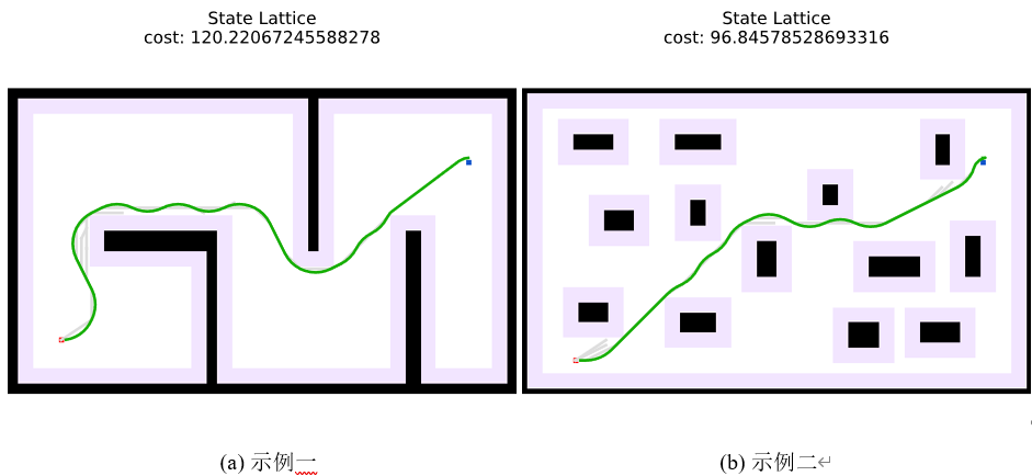
完整工程代码请联系下方博主名片获取
🔥 更多精彩专栏:
👇源码获取 · 技术交流 · 抱团学习 · 咨询分享 请联系👇