机器学习+城市规划第十四期：利用半参数地理加权回归来实现区域带宽不同的规划任务

机器学习+城市规划第十四期：利用半参数地理加权回归来实现区域带宽不同的规划任务

引言

在城市规划中，如何根据不同地区的地理特征来制定有效的规划方案是一个关键问题。不同区域的需求和规律是不同的，因此我们必须考虑到地理空间的差异性。本期博客将介绍如何结合机器学习方法，利用地理加权聚类 （Geographically Weighted Clustering）和半参数地理加权回归（Semi-Parametric Geographically Weighted Regression, SPGWR）来实现城市规划中的区域带宽不同的任务。

我们将通过代码的形式一步步解构整个过程，结合真实的城市数据，帮助大家理解如何在规划过程中处理区域带宽差异问题，并最终实现个性化、优化的规划方案。

地理加权聚类：为什么要加权？

1. 为什么要加权聚类？

传统的聚类方法，如K-means等，通常会根据全局特征对数据进行聚类，而忽略了数据在地理空间上的异质性。而在城市规划中，地理位置对于各类变量的影响至关重要。例如，一个城市的东部和西部，经济发展水平、交通需求、环境污染等因素可能有显著差异。因此，直接应用全局聚类算法可能无法准确地反映不同区域的实际需求。

地理加权聚类能够更好地反映这些空间差异性。通过对每个数据点进行加权处理，我们可以根据每个点的实际因变量（如交通流量、空气污染等）来调整聚类结果，使得相同簇中的数据点具有更强的相似性，并且不同簇之间的差异更加明显。

2. 如何实现加权聚类？

我们使用了DBSCAN（密度基聚类算法），它能够根据每个点的邻域密度来进行聚类。在此基础上，我们根据每个数据点的因变量进行加权复制，以反映不同地区的实际需求。接下来是代码实现过程。

import pandas as pd
import numpy as np
from sklearn.cluster import DBSCAN
import matplotlib.pyplot as plt

# ========== 中文字体设置 ==========
plt.rcParams['font.sans-serif'] = ['SimHei']
plt.rcParams['axes.unicode_minus'] = False

# ========== 读取数据 ==========
df = pd.read_csv('shuju bike.csv', header=None)
df.columns = ['latitude', 'longitude', 'dependent_var', 'independent_var']

# 清洗数据
df['latitude'] = pd.to_numeric(df['latitude'], errors='coerce')
df['longitude'] = pd.to_numeric(df['longitude'], errors='coerce')
df['dependent_var'] = pd.to_numeric(df['dependent_var'], errors='coerce')
df['independent_var'] = pd.to_numeric(df['independent_var'], errors='coerce')
df.dropna(subset=['latitude', 'longitude', 'dependent_var', 'independent_var'], inplace=True)

# ========== 权重复制（加权） ==========
df_weighted = df.loc[df.index.repeat(df['dependent_var'].astype(int))].reset_index(drop=True)

# ========== 转换为弧度坐标 ==========
coords = df_weighted[['latitude', 'longitude']].to_numpy()
coords_rad = np.radians(coords)

# ========== 设置 DBSCAN 参数 ==========
kms_per_radian = 6371.0088
base_eps_km = 5  # 可调：基础 eps，单位为 km
epsilon = base_eps_km / kms_per_radian

# ========== 聚类 ==========
db = DBSCAN(eps=epsilon, min_samples=10, algorithm='ball_tree', metric='haversine')
cluster_labels = db.fit_predict(coords_rad)

# ========== 聚类结果回填到原始 df ==========
df_weighted['cluster'] = cluster_labels

# 按经纬度 + 因变量分组，避免数据重复
df_clustered = df_weighted.groupby(['latitude', 'longitude', 'dependent_var', 'independent_var'], as_index=False).agg({'cluster': 'first'})

# ========== 合并回原始数据 ==========
df_result = pd.merge(df, df_clustered, on=['latitude', 'longitude', 'dependent_var', 'independent_var'], how='left')

# ========== 保存 ==========
output_path = "加权聚类结果.csv"
df_result.to_csv(output_path, index=False, encoding='utf-8-sig')
print("✅ 加权聚类结果已保存至：", output_path)

# ========== 可视化 ==========
plt.figure(figsize=(10, 6))
scatter = plt.scatter(
    df_result['longitude'],
    df_result['latitude'],
    c=df_result['cluster'],
    cmap='tab20',
    s=df_result['dependent_var'] * 10,  # 用大小体现因变量的严重程度
    alpha=0.7
)
plt.xlabel('Longitude')
plt.ylabel('Latitude')
plt.title('地理加权 DBSCAN 聚类（考虑因变量）')
plt.colorbar(scatter, label='Cluster ID')
plt.grid(True)
plt.show()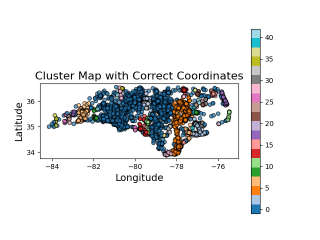

半参数地理加权回归：引入带宽的原因

1. 为什么引入半参数地理加权回归？

在地理空间中，不同地区的数据特征之间可能存在显著差异。例如，在城市的东部地区，温度、湿度等环境变量可能与西部地区的关系完全不同。因此，采用全局回归模型（例如普通最小二乘回归）进行预测可能会忽略这些差异，导致不准确的结果。

半参数地理加权回归（SPGWR）结合了传统回归和地理加权的优势，通过在回归中引入带宽，使得每个区域内的数据点能够根据其空间距离进行加权，从而有效捕捉区域差异。

2. 如何实现半参数地理加权回归？

通过计算每个点与其周围点的地理距离，并根据距离计算权重，我们能够在每个簇内应用不同的回归参数。这使得我们能够根据不同区域的特征，制定个性化的规划方案。

以下是半参数地理加权回归的实现代码：

import pandas as pd
import numpy as np
from sklearn.preprocessing import StandardScaler
from sklearn.metrics import mean_squared_error
import matplotlib.pyplot as plt
from scipy.spatial.distance import cdist
from sklearn.linear_model import LinearRegression
import geopandas as gpd
from shapely.geometry import Point

# 读取加权聚类数据
df = pd.read_csv('加权聚类结果.csv')  # 假设加权聚类结果文件路径

# 处理数据：取出经纬度、因变量和自变量
df['latitude'] = pd.to_numeric(df['latitude'], errors='coerce')
df['longitude'] = pd.to_numeric(df['longitude'], errors='coerce')
df['dependent_var'] = pd.to_numeric(df['dependent_var'], errors='coerce')
df['independent_var'] = pd.to_numeric(df['independent_var'], errors='coerce')
df.dropna(subset=['latitude', 'longitude', 'dependent_var', 'independent_var'], inplace=True)

# 标准化数据
scaler = StandardScaler()
df['dependent_var_scaled'] = scaler.fit_transform(df[['dependent_var']])
df['independent_var_scaled'] = scaler.fit_transform(df[['independent_var']])

# Haversine距离函数
def haversine(lat1, lon1, lat2, lon2):
    R = 6371  # 地球半径（公里）
    phi1, phi2 = np.radians(lat1), np.radians(lat2)
    delta_phi = np.radians(lat2 - lat1)
    delta_lambda = np.radians(lon2 - lon1)

    a = np.sin(delta_phi / 2) ** 2 + np.cos(phi1) * np.cos(phi2) * np.sin(delta_lambda / 2) ** 2
    c = 2 * np.arctan2(np.sqrt(a), np.sqrt(1 - a))

    return R * c

# 计算地理坐标之间的距离矩阵
def compute_distance_matrix(coords):
    return cdist(coords, coords, metric='euclidean')  # 使用欧几里得距离计算地理距离

# 半参数化地理加权回归
def spgwr(coords, X, y, bandwidth):
    dist_matrix = compute_distance_matrix(coords)
    weights = np.exp(-dist_matrix ** 2 / (2 * bandwidth ** 2))  # 高斯权重

    weights = np.diagonal(weights)  # 只选择对角线元素

    model = LinearRegression()
    model.fit(X, y, sample_weight=weights)

    y_pred = model.predict(X)
    residuals = y - y_pred
    RSS = np.sum(residuals ** 2)
    n = len(y)
    k = len(model.coef_)

    log_likelihood = -0.5 * np.sum(np.log(np.maximum(np.abs(residuals), 1e-10)) ** 2)
    AIC = 2 * k - 2 * log_likelihood
    BIC = np.log(n) * k - 2 * log_likelihood

    R2 = model.score(X, y)
    adj_R2 = 1 - (1 - R2) * (n - 1) / (n - k - 1)

    return {
        'RSS': RSS,
        'AIC': AIC,
        'BIC': BIC,
        'R2': R2,
        'Adj_R2': adj_R2,
        'params': model.coef_,
        'intercept': model.intercept_,
        'residuals': residuals
    }, model

# 选择带宽（示例为平均距离）
clusters = df['cluster'].unique()
results = []

for cluster in clusters:
    cluster_data = df[df['cluster'] == cluster]

    coords = cluster_data[['latitude', 'longitude']].to_numpy()
    X = cluster_data[['independent_var_scaled']].to_numpy()
    y = cluster_data['dependent_var_scaled'].to_numpy()

    dist_matrix = compute_distance_matrix(coords)
    bandwidth = np.mean(dist_matrix)

    model_results, model = spgwr(coords, X, y, bandwidth)

    df.loc[df['cluster'] == cluster, 'MGWR_coef_Temperature'] = model_results['params'][0]
    df.loc[df['cluster'] == cluster, 'MGWR_residuals'] = model_results['residuals']

    cluster_results = {
        'cluster': cluster,
        'bandwidth': bandwidth,
        'RSS': model_results['RSS'],
        'AIC': model_results['AIC'],
        'BIC': model_results['BIC'],
        'R2': model_results['R2'],
        'Adj_R2': model_results['Adj_R2'],
        'params': model_results['params'],
        'intercept': model_results['intercept'],
        'mse': mean_squared_error(y, model.predict(X))
    }

    results.append(cluster_results)

# 输出结果
results_df = pd.DataFrame([{
    'Cluster': result['cluster'],
    'Bandwidth': result['bandwidth'],
    'RSS': result['RSS'],
    'AIC': result['AIC'],
    'BIC': result['BIC'],
    'R2': result['R2'],
    'Adj_R2': result['Adj_R2'],
    'MSE': result['mse']
} for result in results])

# 创建 GeoDataFrame
geometry = [Point(xy[1], xy[0]) for xy in zip(df['longitude'], df['latitude'])]
geo_df = gpd.GeoDataFrame(df, geometry=geometry, crs="EPSG:4326")

# 可视化聚类结果
plt.figure(figsize=(12, 6))
geo_df.plot(column='cluster', cmap='tab20', legend=True, markersize=30, alpha=0.7, edgecolor='k')
plt.title('Cluster Map with Correct Coordinates', fontsize=16)
plt.xlabel('Longitude', fontsize=14)
plt.ylabel('Latitude', fontsize=14)
plt.show()

# 保存为 GeoJSON 文件
output_geojson_path = 'spgwr_clusters_corrected.geojson'
geo_df.to_file(output_geojson_path, driver='GeoJSON')

print(f"GeoJSON 文件已保存：{output_geojson_path}")
print(results_df)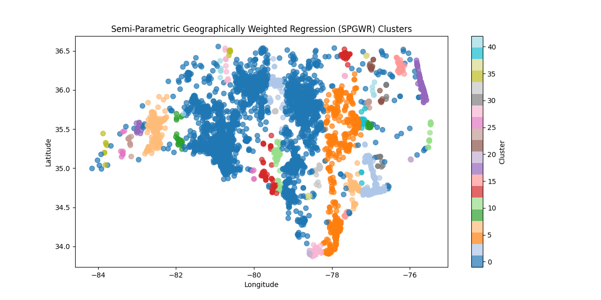

总结

通过使用地理加权聚类 和半参数地理加权回归，我们可以有效地考虑到地理空间上的差异性。在城市规划中，这意味着我们可以为不同区域制定更为精准的规划方案，充分利用地理特征来优化资源分配和决策支持。通过这种方法，我们实现了具有不同区域带宽的个性化规划任务，让城市规划更加科学和合理。

希望大家通过本篇博客，能够深入理解并掌握这些技术，运用在实际的城市规划任务中，提升规划的精准度与效果！

原创声明：本教程由课题组内部教学使用，利用CSDN平台记录，不进行任何商业盈利。