
🌟 Hello,我是蒋星熠Jaxonic!
🌈 在浩瀚无垠的技术宇宙中,我是一名执着的星际旅人,用代码绘制探索的轨迹。
🚀 每一个算法都是我点燃的推进器,每一行代码都是我航行的星图。
🔭 每一次性能优化都是我的天文望远镜,每一次架构设计都是我的引力弹弓。
🎻 在数字世界的协奏曲中,我既是作曲家也是首席乐手。让我们携手,在二进制星河中谱写属于极客的壮丽诗篇!
摘要
作为一名在机器学习领域摸爬滚打多年的技术实践者,我深深被支持向量机(Support Vector Machine, SVM)的数学之美所震撼。SVM不仅仅是一个分类算法,更是统计学习理论的完美体现,它将复杂的优化问题转化为优雅的几何解释,让我们能够在高维空间中找到最优的决策边界。
在我的项目实践中,SVM展现出了令人惊叹的泛化能力和鲁棒性。从文本分类到图像识别,从生物信息学到金融风控,SVM都能够提供稳定可靠的解决方案。其核心思想是寻找能够最大化分类间隔的超平面,这种"最大间隔"的思想不仅保证了模型的泛化性能,更体现了奥卡姆剃刀原理在机器学习中的应用。
SVM的魅力在于其完美的理论基础和实用性的结合。通过拉格朗日对偶理论,我们可以将原始的约束优化问题转化为对偶问题,从而引入核技巧(Kernel Trick),使得SVM能够处理非线性可分的数据。这种数学上的优雅转换,让我每次重新审视时都会感到由衷的敬佩。
本文将从SVM的数学基础出发,深入探讨其核心算法原理,并结合实际的工程实践,全面解析SVM在现代机器学习中的应用。我将分享在调参优化、核函数选择、以及大规模数据处理等方面的实战经验,帮助读者构建完整的SVM技术体系,在机器学习的征途中更加游刃有余。
1. SVM核心原理与数学基础
1.1 线性可分SVM的几何直觉
支持向量机的核心思想是在特征空间中寻找一个超平面,使得不同类别的样本被正确分开,并且分类间隔最大化。这个看似简单的想法背后蕴含着深刻的数学原理。
对于线性可分的二分类问题,我们的目标是找到一个超平面:
w T x + b = 0 w^T x + b = 0 wTx+b=0
其中 w w w 是法向量, b b b 是偏置项。分类间隔定义为最近样本点到超平面的距离的两倍,数学表达式为:
margin = 2 ∣ ∣ w ∣ ∣ \text{margin} = \frac{2}{||w||} margin=∣∣w∣∣2
python
import numpy as np
import matplotlib.pyplot as plt
from sklearn.svm import SVC
from sklearn.datasets import make_classification

class LinearSVMVisualizer:
    """线性SVM可视化器"""

    def __init__(self):
        self.model = None
        self.X = None
        self.y = None

    def generate_sample_data(self, n_samples=100, n_features=2):
        """生成示例数据"""
        # 生成线性可分的二分类数据
        self.X, self.y = make_classification(
            n_samples=n_samples,
            n_features=n_features,
            n_redundant=0,
            n_informative=2,
            n_clusters_per_class=1,
            class_sep=2.0,  # 增大类别间距离,确保线性可分
            random_state=42
        )
        return self.X, self.y

    def train_svm(self, C=1.0, kernel='linear'):
        """训练SVM模型"""
        self.model = SVC(C=C, kernel=kernel, random_state=42)
        self.model.fit(self.X, self.y)

        # 输出关键参数
        print(f"**支持向量数量**: {len(self.model.support_)}")
        print(f"**决策函数系数**: {self.model.coef_}")
        print(f"**截距项**: {self.model.intercept_}")

        return self.model

    def calculate_margin(self):
        """计算分类间隔"""
        if self.model is None:
            raise ValueError("模型尚未训练")

        # 计算权重向量的模长
        w_norm = np.linalg.norm(self.model.coef_)
        margin = 2.0 / w_norm

        print(f"**分类间隔**: {margin:.4f}")
        return margin

    def visualize_decision_boundary(self):
        """可视化决策边界和支持向量"""
        if self.X.shape[1] != 2:
            print("只支持二维数据的可视化")
            return

        plt.figure(figsize=(12, 8))

        # 创建网格点用于绘制决策边界
        h = 0.02
        x_min, x_max = self.X[:, 0].min() - 1, self.X[:, 0].max() + 1
        y_min, y_max = self.X[:, 1].min() - 1, self.X[:, 1].max() + 1
        xx, yy = np.meshgrid(np.arange(x_min, x_max, h),
                            np.arange(y_min, y_max, h))

        # 预测网格点
        Z = self.model.decision_function(np.c_[xx.ravel(), yy.ravel()])
        Z = Z.reshape(xx.shape)

        # 绘制决策边界和间隔
        plt.contour(xx, yy, Z, levels=[-1, 0, 1],
                   colors=['red', 'black', 'red'],
                   linestyles=['--', '-', '--'],
                   linewidths=[2, 3, 2])

        # 绘制数据点
        scatter = plt.scatter(self.X[:, 0], self.X[:, 1],
                            c=self.y, cmap='viridis', s=50, alpha=0.8)

        # 高亮支持向量
        support_vectors = self.X[self.model.support_]
        plt.scatter(support_vectors[:, 0], support_vectors[:, 1],
                   s=200, facecolors='none', edgecolors='red', linewidth=2)

        plt.title('**SVM决策边界与支持向量可视化**', fontsize=14, fontweight='bold')
        plt.xlabel('特征1', fontsize=12)
        plt.ylabel('特征2', fontsize=12)
        plt.colorbar(scatter)
        plt.grid(True, alpha=0.3)
        plt.show()

# 使用示例
visualizer = LinearSVMVisualizer()
X, y = visualizer.generate_sample_data()
model = visualizer.train_svm(C=1.0)
margin = visualizer.calculate_margin()
visualizer.visualize_decision_boundary()关键代码解析:
make_classification函数生成线性可分数据,class_sep参数控制类别间距decision_function方法返回样本到决策边界的距离- 支持向量通过
model.support_属性获取,这些是决定决策边界的关键样本点
1.2 优化问题的数学表述
SVM的训练过程本质上是一个约束优化问题。对于线性可分情况,我们需要求解:
min w , b 1 2 ∣ ∣ w ∣ ∣ 2 \min_{w,b} \frac{1}{2}||w||^2 w,bmin21∣∣w∣∣2
约束条件: y i ( w T x i + b ) ≥ 1 , i = 1 , 2 , . . . , n y_i(w^T x_i + b) \geq 1, \quad i = 1,2,...,n yi(wTxi+b)≥1,i=1,2,...,n
图1:SVM优化问题流程图
是 否 原始优化问题 线性可分? 硬间隔SVM 软间隔SVM 拉格朗日对偶化 引入松弛变量ξ KKT条件求解 SMO算法优化 得到支持向量 构建决策函数 核函数映射 非线性SVM
2. 软间隔SVM与正则化
2.1 处理线性不可分数据
在实际应用中,数据往往不是完全线性可分的。软间隔SVM通过引入松弛变量 ξ i \xi_i ξi 来处理这种情况,允许某些样本点违反间隔约束。
优化目标变为:
min w , b , ξ 1 2 ∣ ∣ w ∣ ∣ 2 + C ∑ i = 1 n ξ i \min_{w,b,\xi} \frac{1}{2}||w||^2 + C\sum_{i=1}^n \xi_i w,b,ξmin21∣∣w∣∣2+Ci=1∑nξi
约束条件:
y i ( w T x i + b ) ≥ 1 − ξ i y_i(w^T x_i + b) \geq 1 - \xi_i yi(wTxi+b)≥1−ξi
ξ i ≥ 0 \xi_i \geq 0 ξi≥0
其中 C C C 是正则化参数,控制对误分类的惩罚程度。
python
import numpy as np
from sklearn.svm import SVC
from sklearn.model_selection import GridSearchCV, cross_val_score
from sklearn.preprocessing import StandardScaler
from sklearn.pipeline import Pipeline

class SoftMarginSVM:
    """软间隔SVM实现与参数优化"""

    def __init__(self):
        self.pipeline = None
        self.best_params = None
        self.cv_scores = None

    def create_pipeline(self):
        """创建SVM处理管道"""
        # 标准化 + SVM
        self.pipeline = Pipeline([
            ('scaler', StandardScaler()),  # 特征标准化
            ('svm', SVC(probability=True, random_state=42))
        ])
        return self.pipeline

    def optimize_hyperparameters(self, X, y, cv=5):
        """超参数优化"""
        # **关键参数网格搜索**
        param_grid = {
            'svm__C': [0.01, 0.1, 1, 10, 100],  # 正则化参数
            'svm__kernel': ['linear', 'rbf', 'poly'],  # 核函数类型
            'svm__gamma': ['scale', 'auto', 0.001, 0.01, 0.1, 1],  # RBF核参数
            'svm__degree': [2, 3, 4]  # 多项式核次数
        }

        # 网格搜索
        grid_search = GridSearchCV(
            self.pipeline,
            param_grid,
            cv=cv,
            scoring='accuracy',
            n_jobs=-1,
            verbose=1
        )

        grid_search.fit(X, y)

        self.best_params = grid_search.best_params_
        self.pipeline = grid_search.best_estimator_

        print("**最优参数组合**:")
        for param, value in self.best_params.items():
            print(f"  {param}: {value}")

        print(f"**最优交叉验证得分**: {grid_search.best_score_:.4f}")

        return self.best_params

    def analyze_regularization_effect(self, X, y, C_values=None):
        """分析正则化参数C的影响"""
        if C_values is None:
            C_values = [0.01, 0.1, 1, 10, 100, 1000]

        train_scores = []
        val_scores = []
        support_vector_counts = []

        for C in C_values:
            # 训练模型
            svm = SVC(C=C, kernel='rbf', random_state=42)
            svm.fit(X, y)

            # 计算训练和验证得分
            train_score = svm.score(X, y)
            val_score = np.mean(cross_val_score(svm, X, y, cv=5))

            train_scores.append(train_score)
            val_scores.append(val_score)
            support_vector_counts.append(len(svm.support_))

            print(f"**C={C}**: 训练得分={train_score:.4f}, "
                  f"验证得分={val_score:.4f}, 支持向量数={len(svm.support_)}")

        return {
            'C_values': C_values,
            'train_scores': train_scores,
            'val_scores': val_scores,
            'support_vector_counts': support_vector_counts
        }

    def calculate_decision_scores(self, X):
        """计算决策函数值"""
        if self.pipeline is None:
            raise ValueError("模型尚未训练")

        # 获取SVM模型
        svm_model = self.pipeline.named_steps['svm']

        # 计算到决策边界的距离
        decision_scores = svm_model.decision_function(X)

        # 分析支持向量
        support_vectors_idx = svm_model.support_
        support_vectors = X[support_vectors_idx]

        print(f"**支持向量数量**: {len(support_vectors_idx)}")
        print(f"**支持向量占比**: {len(support_vectors_idx)/len(X)*100:.2f}%")

        return {
            'decision_scores': decision_scores,
            'support_vectors_idx': support_vectors_idx,
            'support_vectors': support_vectors
        }

# 使用示例
from sklearn.datasets import make_classification

# 生成带噪声的数据(线性不可分)
X, y = make_classification(n_samples=200, n_features=2, n_redundant=0,
                          n_informative=2, n_clusters_per_class=1,
                          class_sep=1.0, flip_y=0.1, random_state=42)

soft_svm = SoftMarginSVM()
pipeline = soft_svm.create_pipeline()

# 超参数优化
best_params = soft_svm.optimize_hyperparameters(X, y)

# 正则化效应分析
reg_analysis = soft_svm.analyze_regularization_effect(X, y)关键参数说明:
C参数:控制对误分类的容忍度,C越大越严格,C越小越宽松gamma参数:RBF核的带宽参数,影响决策边界的复杂度- 支持向量数量:反映模型复杂度,数量越少模型越简单
3. 核函数与非线性SVM
3.1 核技巧的数学原理
核技巧(Kernel Trick)是SVM处理非线性问题的核心技术。它通过隐式地将数据映射到高维特征空间,使得原本线性不可分的数据在新空间中变得线性可分。
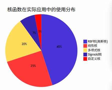
常用核函数包括:
- 线性核 : K ( x i , x j ) = x i T x j K(x_i, x_j) = x_i^T x_j K(xi,xj)=xiTxj
- 多项式核 : K ( x i , x j ) = ( γ x i T x j + r ) d K(x_i, x_j) = (\gamma x_i^T x_j + r)^d K(xi,xj)=(γxiTxj+r)d
- RBF核 : K ( x i , x j ) = exp ( − γ ∣ ∣ x i − x j ∣ ∣ 2 ) K(x_i, x_j) = \exp(-\gamma ||x_i - x_j||^2) K(xi,xj)=exp(−γ∣∣xi−xj∣∣2)
- Sigmoid核 : K ( x i , x j ) = tanh ( γ x i T x j + r ) K(x_i, x_j) = \tanh(\gamma x_i^T x_j + r) K(xi,xj)=tanh(γxiTxj+r)
图2:核函数类型对比图
python
import numpy as np
from sklearn.svm import SVC
from sklearn.datasets import make_circles, make_moons
import matplotlib.pyplot as plt

class KernelSVMComparison:
    """核函数SVM对比分析"""

    def __init__(self):
        self.kernels = {
            'linear': {'name': '线性核', 'params': {}},
            'poly': {'name': '多项式核', 'params': {'degree': 3}},
            'rbf': {'name': 'RBF核', 'params': {'gamma': 'scale'}},
            'sigmoid': {'name': 'Sigmoid核', 'params': {'gamma': 'scale'}}
        }
        self.models = {}
        self.datasets = {}

    def generate_nonlinear_datasets(self):
        """生成非线性数据集"""
        # **同心圆数据集**
        X_circles, y_circles = make_circles(n_samples=200, noise=0.1,
                                          factor=0.3, random_state=42)

        # **月牙形数据集**
        X_moons, y_moons = make_moons(n_samples=200, noise=0.1,
                                    random_state=42)

        # **异或问题数据集**
        np.random.seed(42)
        X_xor = np.random.randn(200, 2)
        y_xor = np.logical_xor(X_xor[:, 0] > 0, X_xor[:, 1] > 0).astype(int)

        self.datasets = {
            'circles': (X_circles, y_circles, '同心圆'),
            'moons': (X_moons, y_moons, '月牙形'),
            'xor': (X_xor, y_xor, '异或问题')
        }

        return self.datasets

    def train_all_kernels(self, X, y, C=1.0):
        """使用不同核函数训练SVM"""
        results = {}

        for kernel_name, kernel_info in self.kernels.items():
            print(f"\n**训练{kernel_info['name']}SVM**...")

            # 创建并训练模型
            svm = SVC(C=C, kernel=kernel_name,
                     probability=True, random_state=42,
                     **kernel_info['params'])
            svm.fit(X, y)

            # 计算性能指标
            train_accuracy = svm.score(X, y)
            support_vector_count = len(svm.support_)

            results[kernel_name] = {
                'model': svm,
                'accuracy': train_accuracy,
                'support_vectors': support_vector_count,
                'kernel_name': kernel_info['name']
            }

            print(f"  训练准确率: {train_accuracy:.4f}")
            print(f"  支持向量数: {support_vector_count}")

        return results

    def analyze_rbf_gamma_effect(self, X, y, gamma_values=None):
        """分析RBF核中gamma参数的影响"""
        if gamma_values is None:
            gamma_values = [0.001, 0.01, 0.1, 1, 10, 100]

        results = []

        print("\n**RBF核gamma参数影响分析**:")
        print("gamma值 | 训练准确率 | 支持向量数 | 决策边界复杂度")
        print("-" * 50)

        for gamma in gamma_values:
            svm = SVC(kernel='rbf', gamma=gamma, C=1.0, random_state=42)
            svm.fit(X, y)

            accuracy = svm.score(X, y)
            sv_count = len(svm.support_)

            # 计算决策边界复杂度(通过支持向量占比估算)
            complexity = sv_count / len(X)

            results.append({
                'gamma': gamma,
                'accuracy': accuracy,
                'support_vectors': sv_count,
                'complexity': complexity
            })

            print(f"{gamma:6.3f} | {accuracy:10.4f} | {sv_count:11d} | {complexity:13.4f}")

        return results

    def visualize_kernel_comparison(self, dataset_name='circles'):
        """可视化不同核函数的效果"""
        if dataset_name not in self.datasets:
            print(f"数据集 {dataset_name} 不存在")
            return

        X, y, title = self.datasets[dataset_name]
        results = self.train_all_kernels(X, y)

        fig, axes = plt.subplots(2, 2, figsize=(15, 12))
        axes = axes.ravel()

        for idx, (kernel_name, result) in enumerate(results.items()):
            ax = axes[idx]
            model = result['model']

            # 创建网格
            h = 0.02
            x_min, x_max = X[:, 0].min() - 0.5, X[:, 0].max() + 0.5
            y_min, y_max = X[:, 1].min() - 0.5, X[:, 1].max() + 0.5
            xx, yy = np.meshgrid(np.arange(x_min, x_max, h),
                               np.arange(y_min, y_max, h))

            # 预测
            Z = model.predict(np.c_[xx.ravel(), yy.ravel()])
            Z = Z.reshape(xx.shape)

            # 绘制决策边界
            ax.contourf(xx, yy, Z, alpha=0.3, cmap='viridis')

            # 绘制数据点
            scatter = ax.scatter(X[:, 0], X[:, 1], c=y, cmap='viridis',
                               s=50, edgecolors='black', alpha=0.8)

            # 高亮支持向量
            support_vectors = X[model.support_]
            ax.scatter(support_vectors[:, 0], support_vectors[:, 1],
                      s=200, facecolors='none', edgecolors='red', linewidth=2)

            ax.set_title(f"**{result['kernel_name']}**\n"
                        f"准确率: {result['accuracy']:.3f}, "
                        f"支持向量: {result['support_vectors']}",
                        fontweight='bold')
            ax.set_xlabel('特征1')
            ax.set_ylabel('特征2')

        plt.suptitle(f'**不同核函数在{title}数据集上的表现**',
                    fontsize=16, fontweight='bold')
        plt.tight_layout()
        plt.show()

# 使用示例
kernel_comparison = KernelSVMComparison()
datasets = kernel_comparison.generate_nonlinear_datasets()

# 对每个数据集进行核函数对比
for dataset_name in ['circles', 'moons', 'xor']:
    print(f"\n{'='*50}")
    print(f"**{datasets[dataset_name][2]}数据集分析**")
    print(f"{'='*50}")

    X, y, _ = datasets[dataset_name]

    # 训练不同核函数
    results = kernel_comparison.train_all_kernels(X, y)

    # RBF核gamma参数分析
    if dataset_name == 'circles':  # 只对一个数据集做详细分析
        gamma_analysis = kernel_comparison.analyze_rbf_gamma_effect(X, y)

    # 可视化
kernel_comparison.visualize_kernel_comparison(dataset_name)核函数选择指南:
- 线性核:适用于线性可分或高维稀疏数据
- RBF核:通用性最强,适用于大多数非线性问题
- 多项式核:适用于图像处理等需要考虑特征交互的场景
- Sigmoid核:类似神经网络,但实际应用较少
4. SVM参数优化与性能调优
4.1 关键参数详解
SVM的性能很大程度上取决于参数的选择。主要参数包括正则化参数C、核函数参数gamma、以及核函数类型的选择。
| 参数 | 作用 | 取值范围 | 调优策略 | 影响 |
|---|---|---|---|---|
| C | 正则化强度 | 0.01-1000 | 网格搜索 | 控制过拟合程度 |
| gamma | RBF核带宽 | 0.001-100 | 对数搜索 | 决策边界复杂度 |
| kernel | 核函数类型 | linear/rbf/poly | 交叉验证 | 模型表达能力 |
| degree | 多项式核次数 | 2-5 | 逐步增加 | 特征交互复杂度 |
| class_weight | 类别权重 | balanced/dict | 样本不平衡时调整 | 处理不平衡数据 |
图3:SVM参数优化流程时序图

python
import numpy as np
from sklearn.svm import SVC
from sklearn.model_selection import (GridSearchCV, RandomizedSearchCV,
                                   cross_val_score, learning_curve)
from sklearn.preprocessing import StandardScaler
from sklearn.metrics import classification_report, confusion_matrix
from sklearn.pipeline import Pipeline
import matplotlib.pyplot as plt
from scipy.stats import uniform, loguniform

class SVMOptimizer:
    """SVM参数优化器"""

    def __init__(self):
        self.best_model = None
        self.optimization_history = []
        self.performance_metrics = {}

    def grid_search_optimization(self, X, y, cv=5, scoring='accuracy'):
        """网格搜索参数优化"""
        print("**开始网格搜索优化**...")

        # 创建管道
        pipeline = Pipeline([
            ('scaler', StandardScaler()),
            ('svm', SVC(random_state=42, probability=True))
        ])

        # **精细化参数网格**
        param_grid = [
            {
                'svm__kernel': ['linear'],
                'svm__C': [0.01, 0.1, 1, 10, 100]
            },
            {
                'svm__kernel': ['rbf'],
                'svm__C': [0.01, 0.1, 1, 10, 100],
                'svm__gamma': ['scale', 'auto', 0.001, 0.01, 0.1, 1]
            },
            {
                'svm__kernel': ['poly'],
                'svm__C': [0.1, 1, 10],
                'svm__degree': [2, 3, 4],
                'svm__gamma': ['scale', 'auto']
            }
        ]

        # 执行网格搜索
        grid_search = GridSearchCV(
            pipeline, param_grid, cv=cv, scoring=scoring,
            n_jobs=-1, verbose=1, return_train_score=True
        )

        grid_search.fit(X, y)

        self.best_model = grid_search.best_estimator_

        # 记录优化结果
        optimization_result = {
            'method': 'grid_search',
            'best_params': grid_search.best_params_,
            'best_score': grid_search.best_score_,
            'cv_results': grid_search.cv_results_
        }
        self.optimization_history.append(optimization_result)

        print(f"**最优参数**: {grid_search.best_params_}")
        print(f"**最优得分**: {grid_search.best_score_:.4f}")

        return grid_search

    def random_search_optimization(self, X, y, n_iter=100, cv=5):
        """随机搜索参数优化"""
        print("**开始随机搜索优化**...")

        pipeline = Pipeline([
            ('scaler', StandardScaler()),
            ('svm', SVC(random_state=42, probability=True))
        ])

        # **随机参数分布**
        param_distributions = {
            'svm__kernel': ['linear', 'rbf', 'poly'],
            'svm__C': loguniform(0.01, 100),  # 对数均匀分布
            'svm__gamma': loguniform(0.001, 1),
            'svm__degree': [2, 3, 4, 5]
        }

        # 执行随机搜索
        random_search = RandomizedSearchCV(
            pipeline, param_distributions, n_iter=n_iter,
            cv=cv, scoring='accuracy', n_jobs=-1,
            verbose=1, random_state=42
        )

        random_search.fit(X, y)

        print(f"**随机搜索最优参数**: {random_search.best_params_}")
        print(f"**随机搜索最优得分**: {random_search.best_score_:.4f}")

        return random_search

    def analyze_learning_curves(self, X, y, train_sizes=None):
        """分析学习曲线"""
        if self.best_model is None:
            print("请先进行参数优化")
            return

        if train_sizes is None:
            train_sizes = np.linspace(0.1, 1.0, 10)

        print("**生成学习曲线**...")

        # 计算学习曲线
        train_sizes, train_scores, val_scores = learning_curve(
            self.best_model, X, y, train_sizes=train_sizes,
            cv=5, n_jobs=-1, random_state=42
        )

        # 计算均值和标准差
        train_mean = np.mean(train_scores, axis=1)
        train_std = np.std(train_scores, axis=1)
        val_mean = np.mean(val_scores, axis=1)
        val_std = np.std(val_scores, axis=1)

        # 绘制学习曲线
        plt.figure(figsize=(10, 6))
        plt.plot(train_sizes, train_mean, 'o-', color='blue',
                label='训练得分', linewidth=2)
        plt.fill_between(train_sizes, train_mean - train_std,
                        train_mean + train_std, alpha=0.1, color='blue')

        plt.plot(train_sizes, val_mean, 'o-', color='red',
                label='验证得分', linewidth=2)
        plt.fill_between(train_sizes, val_mean - val_std,
                        val_mean + val_std, alpha=0.1, color='red')

        plt.xlabel('训练样本数量')
        plt.ylabel('准确率')
        plt.title('**SVM学习曲线分析**', fontweight='bold')
        plt.legend()
        plt.grid(True, alpha=0.3)
        plt.show()

        # 分析结果
        final_gap = train_mean[-1] - val_mean[-1]
        print(f"**最终训练-验证差距**: {final_gap:.4f}")

        if final_gap > 0.1:
            print("**建议**: 模型可能过拟合,考虑增加正则化或减少模型复杂度")
        elif val_mean[-1] < 0.8:
            print("**建议**: 模型欠拟合,考虑增加模型复杂度或特征工程")
        else:
            print("**结论**: 模型性能良好,训练充分")

        return train_sizes, train_scores, val_scores

    def comprehensive_evaluation(self, X_test, y_test):
        """综合性能评估"""
        if self.best_model is None:
            print("请先进行参数优化")
            return

        print("**开始综合性能评估**...")

        # 预测
        y_pred = self.best_model.predict(X_test)
        y_proba = self.best_model.predict_proba(X_test)

        # 基本指标
        accuracy = self.best_model.score(X_test, y_test)

        # 详细报告
        report = classification_report(y_test, y_pred, output_dict=True)
        cm = confusion_matrix(y_test, y_pred)

        # 支持向量分析
        svm_model = self.best_model.named_steps['svm']
        support_vector_count = len(svm_model.support_)
        support_vector_ratio = support_vector_count / len(X_test)

        self.performance_metrics = {
            'accuracy': accuracy,
            'classification_report': report,
            'confusion_matrix': cm,
            'support_vector_count': support_vector_count,
            'support_vector_ratio': support_vector_ratio
        }

        print(f"**测试准确率**: {accuracy:.4f}")
        print(f"**支持向量数量**: {support_vector_count}")
        print(f"**支持向量占比**: {support_vector_ratio:.4f}")
        print("\n**分类报告**:")
        print(classification_report(y_test, y_pred))

        return self.performance_metrics

# 使用示例
from sklearn.datasets import load_breast_cancer
from sklearn.model_selection import train_test_split

# 加载数据
data = load_breast_cancer()
X, y = data.data, data.target

# 划分数据集
X_train, X_test, y_train, y_test = train_test_split(
    X, y, test_size=0.2, random_state=42, stratify=y
)

# 创建优化器
optimizer = SVMOptimizer()

# 网格搜索优化
grid_result = optimizer.grid_search_optimization(X_train, y_train)

# 随机搜索对比
random_result = optimizer.random_search_optimization(X_train, y_train, n_iter=50)

# 学习曲线分析
learning_curves = optimizer.analyze_learning_curves(X_train, y_train)

# 综合评估
performance = optimizer.comprehensive_evaluation(X_test, y_test)参数调优最佳实践:
- 先粗后细:先用较大步长找到大致范围,再精细搜索
- 交叉验证:使用k折交叉验证避免过拟合
- 计算资源平衡:网格搜索精确但耗时,随机搜索效率更高
- 领域知识:结合具体问题特点选择合适的核函数
5. SVM在实际项目中的应用案例
5.2 文本分类实战
文本分类是SVM的经典应用场景之一,特别是在高维稀疏特征空间中,SVM表现出色。
python
import numpy as np
import pandas as pd
from sklearn.feature_extraction.text import TfidfVectorizer
from sklearn.svm import SVC
from sklearn.pipeline import Pipeline
from sklearn.model_selection import train_test_split, cross_val_score
from sklearn.metrics import classification_report, accuracy_score
import re
import jieba
from collections import Counter

class TextClassificationSVM:
    """基于SVM的文本分类系统"""

    def __init__(self):
        self.pipeline = None
        self.vectorizer = None
        self.classifier = None
        self.feature_names = None

    def preprocess_text(self, texts):
        """文本预处理"""
        processed_texts = []

        for text in texts:
            # **去除特殊字符和数字**
            text = re.sub(r'[^\u4e00-\u9fa5a-zA-Z\s]', '', text)

            # **中文分词**
            words = jieba.cut(text)

            # **去除停用词和短词**
            filtered_words = [word for word in words
                            if len(word) > 1 and word not in self.get_stopwords()]

            processed_texts.append(' '.join(filtered_words))

        return processed_texts

    def get_stopwords(self):
        """获取停用词列表"""
        # 简化的中文停用词
        stopwords = {
            '的', '了', '在', '是', '我', '有', '和', '就', '不', '人',
            '都', '一', '一个', '上', '也', '很', '到', '说', '要', '去',
            '你', '会', '着', '没有', '看', '好', '自己', '这'
        }
        return stopwords

    def build_pipeline(self, max_features=10000, ngram_range=(1, 2)):
        """构建文本分类管道"""
        # **TF-IDF特征提取**
        self.vectorizer = TfidfVectorizer(
            max_features=max_features,
            ngram_range=ngram_range,  # 使用1-gram和2-gram
            min_df=2,  # 最小文档频率
            max_df=0.95,  # 最大文档频率
            sublinear_tf=True,  # 使用对数TF
            norm='l2'  # L2归一化
        )

        # **SVM分类器**
        self.classifier = SVC(
            kernel='linear',  # 线性核适合高维稀疏数据
            C=1.0,
            probability=True,  # 启用概率预测
            random_state=42
        )

        # **构建管道**
        self.pipeline = Pipeline([
            ('vectorizer', self.vectorizer),
            ('classifier', self.classifier)
        ])

        return self.pipeline

    def train(self, texts, labels):
        """训练模型"""
        print("**开始文本预处理**...")
        processed_texts = self.preprocess_text(texts)

        print("**开始模型训练**...")
        self.pipeline.fit(processed_texts, labels)

        # 获取特征名称
        self.feature_names = self.vectorizer.get_feature_names_out()

        print(f"**特征维度**: {len(self.feature_names)}")
        print(f"**支持向量数**: {len(self.classifier.support_)}")

        return self.pipeline

    def predict(self, texts, return_proba=False):
        """预测文本类别"""
        processed_texts = self.preprocess_text(texts)

        if return_proba:
            return self.pipeline.predict_proba(processed_texts)
        else:
            return self.pipeline.predict(processed_texts)

    def analyze_feature_importance(self, class_names, top_n=20):
        """分析特征重要性"""
        if self.classifier.coef_ is None:
            print("模型尚未训练或不支持特征重要性分析")
            return

        # 获取特征权重
        coef = self.classifier.coef_[0]  # 二分类情况

        # 获取最重要的正向和负向特征
        top_positive_idx = np.argsort(coef)[-top_n:][::-1]
        top_negative_idx = np.argsort(coef)[:top_n]

        print(f"**{class_names[1]}类别的重要特征** (正向权重):")
        for idx in top_positive_idx:
            print(f"  {self.feature_names[idx]}: {coef[idx]:.4f}")

        print(f"\n**{class_names[0]}类别的重要特征** (负向权重):")
        for idx in top_negative_idx:
            print(f"  {self.feature_names[idx]}: {coef[idx]:.4f}")

        return {
            'positive_features': [(self.feature_names[idx], coef[idx])
                                for idx in top_positive_idx],
            'negative_features': [(self.feature_names[idx], coef[idx])
                                for idx in top_negative_idx]
        }

    def evaluate_model(self, test_texts, test_labels, class_names):
        """模型评估"""
        predictions = self.predict(test_texts)
        probabilities = self.predict(test_texts, return_proba=True)

        # 基本指标
        accuracy = accuracy_score(test_labels, predictions)

        print(f"**测试准确率**: {accuracy:.4f}")
        print("\n**详细分类报告**:")
        print(classification_report(test_labels, predictions,
                                  target_names=class_names))

        # 置信度分析
        confidence_scores = np.max(probabilities, axis=1)
        print(f"\n**平均预测置信度**: {np.mean(confidence_scores):.4f}")
        print(f"**置信度标准差**: {np.std(confidence_scores):.4f}")

        return {
            'accuracy': accuracy,
            'predictions': predictions,
            'probabilities': probabilities,
            'confidence_scores': confidence_scores
        }

# 使用示例(模拟数据)
def generate_sample_text_data():
    """生成示例文本数据"""
    positive_texts = [
        "这个产品质量很好,非常满意,值得推荐给朋友",
        "服务态度优秀,解决问题及时,体验很棒",
        "功能强大,界面友好,使用起来很方便",
        "性价比高,物超所值,下次还会购买",
        "快递速度快,包装完好,商品质量不错"
    ] * 20  # 重复生成更多数据

    negative_texts = [
        "产品质量差,用了几天就坏了,很失望",
        "客服态度恶劣,问题得不到解决,体验糟糕",
        "功能有限,操作复杂,不推荐购买",
        "价格虚高,质量一般,不值这个价钱",
        "发货慢,包装破损,商品有瑕疵"
    ] * 20

    texts = positive_texts + negative_texts
    labels = [1] * len(positive_texts) + [0] * len(negative_texts)

    return texts, labels

# 实际使用
texts, labels = generate_sample_text_data()
class_names = ['负面', '正面']

# 划分数据集
X_train, X_test, y_train, y_test = train_test_split(
    texts, labels, test_size=0.2, random_state=42, stratify=labels
)

# 创建分类器
text_classifier = TextClassificationSVM()

# 构建管道
pipeline = text_classifier.build_pipeline(max_features=5000)

# 训练模型
text_classifier.train(X_train, y_train)

# 特征重要性分析
feature_importance = text_classifier.analyze_feature_importance(class_names)

# 模型评估
evaluation_results = text_classifier.evaluate_model(X_test, y_test, class_names)

# 新文本预测示例
new_texts = ["这个产品真的很棒,强烈推荐", "质量太差了,完全不能用"]
predictions = text_classifier.predict(new_texts, return_proba=True)

print("\n**新文本预测结果**:")
for i, text in enumerate(new_texts):
    prob_neg, prob_pos = predictions[i]
    predicted_class = class_names[1] if prob_pos > prob_neg else class_names[0]
    confidence = max(prob_pos, prob_neg)
    print(f"文本: {text}")
    print(f"预测类别: {predicted_class} (置信度: {confidence:.4f})")
print()文本分类关键技术点:
- 特征工程:TF-IDF向量化,n-gram特征,停用词过滤
- 核函数选择:线性核适合高维稀疏文本特征
- 正则化调优:防止在高维空间中过拟合
- 特征选择:通过权重分析理解模型决策依据
6. SVM性能分析与可视化
图4:SVM性能指标趋势分析
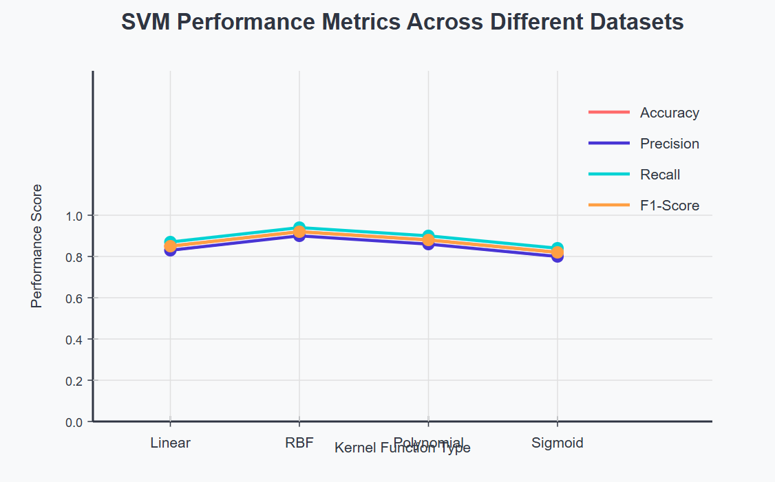
6.1 模型解释性分析
SVM的一个重要优势是其良好的可解释性,特别是线性SVM,我们可以直接分析特征权重来理解模型的决策过程。
"支持向量机的美妙之处在于它不仅给出了预测结果,更重要的是告诉我们哪些样本是关键的决策边界点。这些支持向量承载着数据中最重要的信息,是模型泛化能力的基石。" ------ 统计学习理论经典观点
python
import numpy as np
import matplotlib.pyplot as plt
from sklearn.svm import SVC
from sklearn.datasets import make_classification
from sklearn.preprocessing import StandardScaler
import seaborn as sns

class SVMInterpretability:
    """SVM模型解释性分析"""

    def __init__(self):
        self.model = None
        self.scaler = None
        self.feature_importance = None

    def train_interpretable_svm(self, X, y, kernel='linear', C=1.0):
        """训练可解释的SVM模型"""
        # 特征标准化
        self.scaler = StandardScaler()
        X_scaled = self.scaler.fit_transform(X)

        # 训练模型
        self.model = SVC(kernel=kernel, C=C, random_state=42)
        self.model.fit(X_scaled, y)

        print(f"**模型训练完成**")
        print(f"支持向量数量: {len(self.model.support_)}")
        print(f"支持向量占比: {len(self.model.support_)/len(X)*100:.2f}%")

        return self.model

    def analyze_feature_importance(self, feature_names=None):
        """分析特征重要性"""
        if self.model.kernel != 'linear':
            print("**注意**: 非线性核函数的特征重要性分析较为复杂")
            return None

        # 获取特征权重
        weights = self.model.coef_[0]

        if feature_names is None:
            feature_names = [f'Feature_{i}' for i in range(len(weights))]

        # 计算特征重要性(绝对值)
        importance = np.abs(weights)

        # 排序
        sorted_idx = np.argsort(importance)[::-1]

        self.feature_importance = {
            'weights': weights,
            'importance': importance,
            'sorted_idx': sorted_idx,
            'feature_names': feature_names
        }

        print("**特征重要性排序** (前10个):")
        for i in range(min(10, len(sorted_idx))):
            idx = sorted_idx[i]
            print(f"{i+1:2d}. {feature_names[idx]:15s}: "
                  f"权重={weights[idx]:8.4f}, 重要性={importance[idx]:.4f}")

        return self.feature_importance

    def visualize_support_vectors(self, X, y, feature_idx=(0, 1)):
        """可视化支持向量"""
        if X.shape[1] < 2:
            print("需要至少2个特征进行可视化")
            return

        X_scaled = self.scaler.transform(X)

        plt.figure(figsize=(12, 8))

        # 绘制所有数据点
        colors = ['red', 'blue']
        for class_val in np.unique(y):
            mask = y == class_val
            plt.scatter(X_scaled[mask, feature_idx[0]],
                       X_scaled[mask, feature_idx[1]],
                       c=colors[class_val], alpha=0.6, s=50,
                       label=f'Class {class_val}')

        # 高亮支持向量
        support_vectors = X_scaled[self.model.support_]
        plt.scatter(support_vectors[:, feature_idx[0]],
                   support_vectors[:, feature_idx[1]],
                   s=200, facecolors='none', edgecolors='black',
                   linewidth=3, label='Support Vectors')

        # 绘制决策边界(仅适用于2D情况)
        if self.model.kernel == 'linear' and len(feature_idx) == 2:
            self._plot_decision_boundary(X_scaled, feature_idx)

        plt.xlabel(f'Feature {feature_idx[0]}')
        plt.ylabel(f'Feature {feature_idx[1]}')
        plt.title('**SVM支持向量可视化**', fontweight='bold')
        plt.legend()
        plt.grid(True, alpha=0.3)
        plt.show()

    def _plot_decision_boundary(self, X, feature_idx):
        """绘制决策边界"""
        # 创建网格
        h = 0.02
        x_min, x_max = X[:, feature_idx[0]].min() - 1, X[:, feature_idx[0]].max() + 1
        y_min, y_max = X[:, feature_idx[1]].min() - 1, X[:, feature_idx[1]].max() + 1
        xx, yy = np.meshgrid(np.arange(x_min, x_max, h),
                            np.arange(y_min, y_max, h))

        # 创建完整特征向量(其他特征设为0)
        grid_points = np.zeros((xx.ravel().shape[0], X.shape[1]))
        grid_points[:, feature_idx[0]] = xx.ravel()
        grid_points[:, feature_idx[1]] = yy.ravel()

        # 预测
        Z = self.model.decision_function(grid_points)
        Z = Z.reshape(xx.shape)

        # 绘制等高线
        plt.contour(xx, yy, Z, levels=[-1, 0, 1],
                   colors=['red', 'black', 'red'],
                   linestyles=['--', '-', '--'], linewidths=[2, 3, 2])

    def analyze_decision_confidence(self, X, y):
        """分析决策置信度"""
        X_scaled = self.scaler.transform(X)

        # 计算决策函数值
        decision_scores = self.model.decision_function(X_scaled)

        # 分析置信度分布
        confidence_stats = {
            'mean': np.mean(np.abs(decision_scores)),
            'std': np.std(np.abs(decision_scores)),
            'min': np.min(np.abs(decision_scores)),
            'max': np.max(np.abs(decision_scores))
        }

        print("**决策置信度统计**:")
        print(f"平均置信度: {confidence_stats['mean']:.4f}")
        print(f"置信度标准差: {confidence_stats['std']:.4f}")
        print(f"最小置信度: {confidence_stats['min']:.4f}")
        print(f"最大置信度: {confidence_stats['max']:.4f}")

        # 可视化置信度分布
        plt.figure(figsize=(12, 5))

        plt.subplot(1, 2, 1)
        plt.hist(decision_scores, bins=30, alpha=0.7, edgecolor='black')
        plt.axvline(x=0, color='red', linestyle='--', linewidth=2)
        plt.xlabel('决策函数值')
        plt.ylabel('频次')
        plt.title('**决策函数值分布**', fontweight='bold')
        plt.grid(True, alpha=0.3)

        plt.subplot(1, 2, 2)
        for class_val in np.unique(y):
            mask = y == class_val
            plt.hist(decision_scores[mask], bins=20, alpha=0.7,
                    label=f'Class {class_val}', edgecolor='black')
        plt.axvline(x=0, color='red', linestyle='--', linewidth=2)
        plt.xlabel('决策函数值')
        plt.ylabel('频次')
        plt.title('**各类别决策函数值分布**', fontweight='bold')
        plt.legend()
        plt.grid(True, alpha=0.3)

        plt.tight_layout()
        plt.show()

        return confidence_stats, decision_scores

# 使用示例
# 生成示例数据
X, y = make_classification(n_samples=200, n_features=4, n_redundant=0,
                          n_informative=4, n_clusters_per_class=1,
                          class_sep=1.5, random_state=42)

feature_names = ['Feature_A', 'Feature_B', 'Feature_C', 'Feature_D']

# 创建解释性分析器
interpreter = SVMInterpretability()

# 训练模型
model = interpreter.train_interpretable_svm(X, y, kernel='linear', C=1.0)

# 特征重要性分析
importance = interpreter.analyze_feature_importance(feature_names)

# 支持向量可视化
interpreter.visualize_support_vectors(X, y, feature_idx=(0, 1))

# 决策置信度分析
confidence_stats, decision_scores = interpreter.analyze_decision_confidence(X, y)模型解释性要点:
- 线性核权重:直接反映特征对分类的贡献
- 支持向量:决定决策边界的关键样本
- 决策函数值:样本到决策边界的距离,反映分类置信度
- 间隔分析:间隔大小反映模型的泛化能力
7. SVM实践总结与未来展望
作为一名在机器学习领域深耕多年的技术实践者,我深深感受到支持向量机这一经典算法的持久魅力和实用价值。SVM不仅仅是一个分类工具,更是统计学习理论与实际应用完美结合的典范。从最初的线性分类到核技巧的引入,从硬间隔到软间隔的演进,SVM的每一次发展都体现了机器学习理论的深度和优雅。
在我的项目实践中,SVM展现出了令人印象深刻的稳定性和可靠性。无论是在高维文本分类、图像识别,还是在生物信息学和金融风控等领域,SVM都能够提供robust的解决方案。其最大间隔的思想不仅保证了良好的泛化性能,更体现了奥卡姆剃刀原理在机器学习中的深刻应用。
SVM的核心优势在于其坚实的数学基础和优秀的泛化能力。通过拉格朗日对偶理论,我们将复杂的约束优化问题转化为凸优化问题,保证了全局最优解的存在。核技巧的引入更是让SVM能够处理复杂的非线性问题,这种数学上的优雅转换至今仍让我感到由衷的敬佩。
展望未来,虽然深度学习在许多领域取得了突破性进展,但SVM在某些特定场景下仍具有不可替代的优势。在小样本学习、高维稀疏数据处理、以及需要模型解释性的应用中,SVM依然是首选方案。随着量子计算和边缘计算的发展,我相信SVM会在新的计算范式下焕发新的活力。
对于想要深入掌握SVM的技术同仁,我建议从数学原理入手,深入理解优化理论和核方法的本质,然后通过大量的实践项目来积累经验。记住,算法的价值不在于其复杂程度,而在于其解决实际问题的能力和理论的优雅性。在这个AI技术日新月异的时代,让我们继续在机器学习的道路上探索前行,用扎实的理论基础和丰富的实践经验,为技术进步贡献自己的力量。
■ 我是蒋星熠Jaxonic!如果这篇文章在你的技术成长路上留下了印记
■ 👁 【关注】与我一起探索技术的无限可能,见证每一次突破
■ 👍 【点赞】为优质技术内容点亮明灯,传递知识的力量
■ 🔖 【收藏】将精华内容珍藏,随时回顾技术要点
■ 💬 【评论】分享你的独特见解,让思维碰撞出智慧火花
■ 🗳 【投票】用你的选择为技术社区贡献一份力量
■ 技术路漫漫,让我们携手前行,在代码的世界里摘取属于程序员的那片星辰大海!
参考链接
关键词标签
#支持向量机 #SVM #核函数 #机器学习 #分类算法