目录
[一、Load Data 加载数据](#一、Load Data 加载数据)
[二、Explore Data 探索数据](#二、Explore Data 探索数据)
[三、OLS analysis 普通最小二乘分析](#三、OLS analysis 普通最小二乘分析)
[1-Day Returns](#1-Day Returns)
[5-Day Returns](#5-Day Returns)
[四、Obtain the residuals 计算残差](#四、Obtain the residuals 计算残差)
[residuals analysis 残差分析](#residuals analysis 残差分析)
[10-Day Returns](#10-Day Returns)
[Monthly Returns](#Monthly Returns)
Statistical inference of stock returns with linear regression
这些需要先从0703中构建数据,然后再这一篇。
一、Load Data 加载数据
python
import warnings
warnings.filterwarnings('ignore')

%matplotlib inline

import pandas as pd

from statsmodels.api import OLS, add_constant, graphics
from statsmodels.graphics.tsaplots import plot_acf
from scipy.stats import norm

import seaborn as sns
import matplotlib.pyplot as plt

sns.set_style('whitegrid')
idx = pd.IndexSlice
python
# Load Data
with pd.HDFStore('data.h5') as store:
    data = (store['model_data']
            .dropna()
            .drop(['open', 'close', 'low', 'high'], axis=1))

# Select Investment Universe
data = data[data.dollar_vol_rank<100]
data.info(show_counts=True)
输出:
python
<class 'pandas.core.frame.DataFrame'>
MultiIndex: 109434 entries, ('AAL', Timestamp('2013-07-26 00:00:00')) to ('YUM', Timestamp('2015-11-03 00:00:00'))
Data columns (total 65 columns):
 #   Column                 Non-Null Count   Dtype
---  ------                 --------------   -----
 0   volume                 109434 non-null  float64
 1   dollar_vol             109434 non-null  float64
 2   dollar_vol_1m          109434 non-null  float64
 3   dollar_vol_rank        109434 non-null  float64
 4   rsi                    109434 non-null  float64
 5   bb_high                109434 non-null  float64
 6   bb_low                 109434 non-null  float64
 7   atr                    109434 non-null  float64
 8   macd                   109434 non-null  float64
 9   return_1d              109434 non-null  float64
 10  return_5d              109434 non-null  float64
 11  return_10d             109434 non-null  float64
 12  return_21d             109434 non-null  float64
 13  return_42d             109434 non-null  float64
 14  return_63d             109434 non-null  float64
 15  return_1d_lag1         109434 non-null  float64
 16  return_5d_lag1         109434 non-null  float64
 17  return_10d_lag1        109434 non-null  float64
 18  return_21d_lag1        109434 non-null  float64
 19  return_1d_lag2         109434 non-null  float64
 20  return_5d_lag2         109434 non-null  float64
 21  return_10d_lag2        109434 non-null  float64
 22  return_21d_lag2        109434 non-null  float64
 23  return_1d_lag3         109434 non-null  float64
 24  return_5d_lag3         109434 non-null  float64
 25  return_10d_lag3        109434 non-null  float64
 26  return_21d_lag3        109434 non-null  float64
 27  return_1d_lag4         109434 non-null  float64
 28  return_5d_lag4         109434 non-null  float64
 29  return_10d_lag4        109434 non-null  float64
 30  return_21d_lag4        109434 non-null  float64
 31  return_1d_lag5         109434 non-null  float64
 32  return_5d_lag5         109434 non-null  float64
 33  return_10d_lag5        109434 non-null  float64
 34  return_21d_lag5        109434 non-null  float64
 35  target_1d              109434 non-null  float64
 36  target_5d              109434 non-null  float64
 37  target_10d             109434 non-null  float64
 38  target_21d             109434 non-null  float64
 39  year_2014              109434 non-null  bool
 40  year_2015              109434 non-null  bool
 41  year_2016              109434 non-null  bool
 42  year_2017              109434 non-null  bool
 43  month_2                109434 non-null  bool
 44  month_3                109434 non-null  bool
 45  month_4                109434 non-null  bool
 46  month_5                109434 non-null  bool
 47  month_6                109434 non-null  bool
 48  month_7                109434 non-null  bool
 49  month_8                109434 non-null  bool
 50  month_9                109434 non-null  bool
 51  month_10               109434 non-null  bool
 52  month_11               109434 non-null  bool
 53  month_12               109434 non-null  bool
 54  capital_goods          109434 non-null  bool
 55  consumer_durables      109434 non-null  bool
 56  consumer_non-durables  109434 non-null  bool
 57  consumer_services      109434 non-null  bool
 58  energy                 109434 non-null  bool
 59  finance                109434 non-null  bool
 60  health_care            109434 non-null  bool
 61  miscellaneous          109434 non-null  bool
 62  public_utilities       109434 non-null  bool
 63  technology             109434 non-null  bool
 64  transportation         109434 non-null  bool
dtypes: bool(26), float64(39)
memory usage: 36.5+ MB
Create Model Data
python
y = data.filter(like='target')
X = data.drop(y.columns, axis=1)
X = X.drop(['dollar_vol', 'dollar_vol_rank', 'volume', 'consumer_durables'], axis=1)
如果这里报错的话,要修改上一节0704的代码:
python
prices['sector'] = prices['sector'].str.lower().str.replace(' ', '_')  # add code;增加的代码

prices.assign(sector=pd.factorize(prices.sector, sort=True)[0]).to_hdf('data.h5', 'model_data/no_dummies')
prices = pd.get_dummies(prices,
                        columns=['year', 'month', 'sector'],
                        prefix=['year', 'month', ''],
                        prefix_sep=['_', '_', ''],
                        drop_first=True)
prices.info(show_counts=True)
二、Explore Data 探索数据
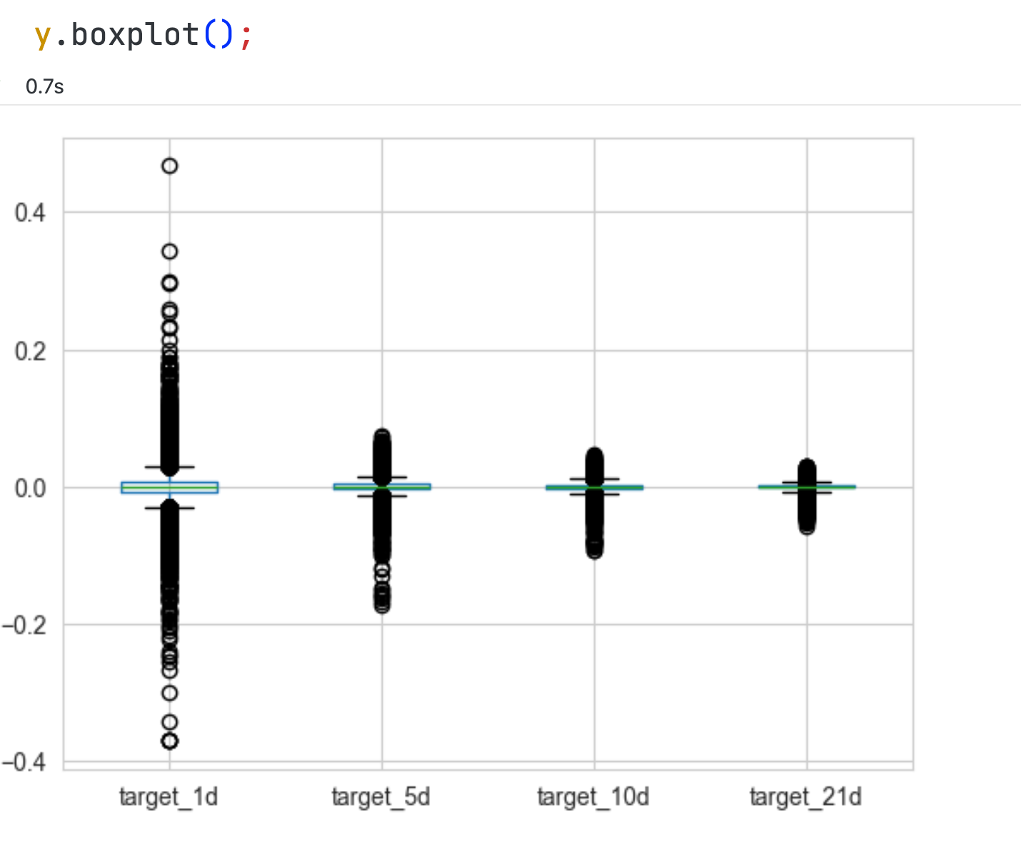
python
sns.clustermap(y.corr(), cmap=sns.diverging_palette(h_neg=20, h_pos=220), center=0, annot=True, fmt='.2%');
python
sns.clustermap(X.corr(), cmap=sns.diverging_palette(h_neg=20, h_pos=220), center=0);
plt.gcf().set_size_inches((14, 14))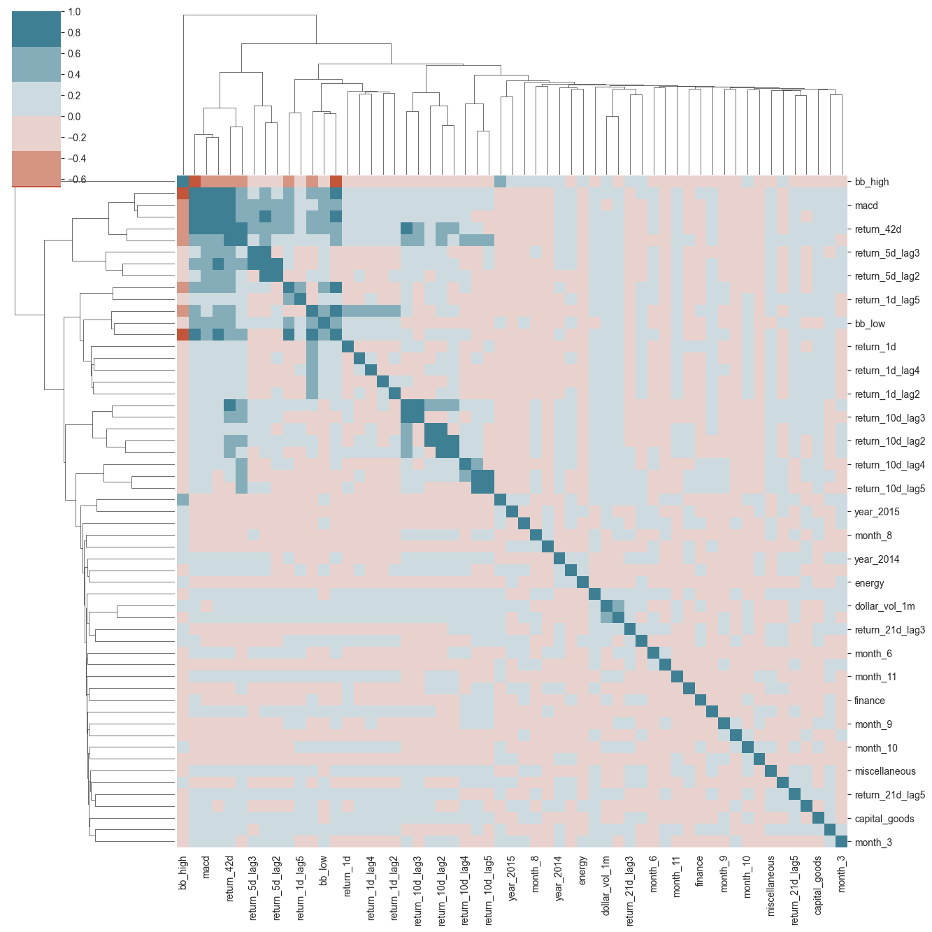
热力图结论:
热力图显示了特征之间的相关性。
相关系数的范围在-1到1之间,值越接近1或-1,说明特征之间的相关性越强。
相关系数为0说明特征之间没有相关性。
Conclusion of heat map:
The heatmap shows the correlation between features.
The range of the correlation coefficient is between -1 and 1. The closer the value is to 1 or -1, the stronger the correlation between the features.
A correlation coefficient of 0 indicates that there is no correlation between the features.
python
corr_mat = X.corr().stack().reset_index()
corr_mat.columns=['var1', 'var2', 'corr']
corr_mat = corr_mat[corr_mat.var1!=corr_mat.var2].sort_values(by='corr', ascending=False)

# corr_mat.head().append(corr_mat.tail())  old code is bad; 作者原始代码已经不行了
pd.concat([corr_mat.head(), corr_mat.tail()])  # pandas ≥ 2.0 good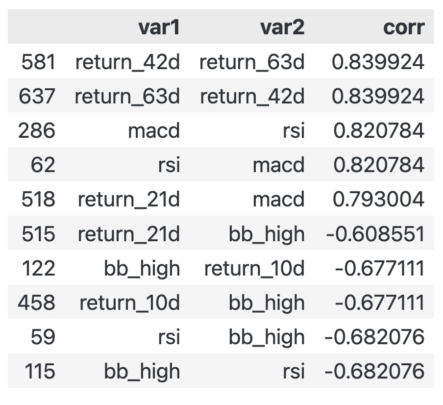
三、OLS analysis 普通最小二乘分析
Linear Regression for Statistical Inference: OLS with statsmodels
用statsmodels库进行线性回归分析,OLS线性回归
Ticker-wise standardization
statsmodels warns of high design matrix condition numbers. This can arise when the variables are not standardized and the Eigenvalues differ due to scaling. The following step avoids this warning.
python
sectors = X.iloc[:, -10:]
X = (X.drop(sectors.columns, axis=1)
     .groupby(level='ticker')
     .transform(lambda x: (x - x.mean()) / x.std())
    .join(sectors)
    .fillna(0))
1-Day Returns
python
target = 'target_1d'
# this is MultiIndex
# model = OLS(endog=y[target], exog=add_constant(X))      # old code is bad; 老代码失效
X = X.astype(float)
model = OLS(endog=y[target], exog=add_constant(X))    # this is good.
trained_model = model.fit()
print(trained_model.summary())

# R-squared is only 0.009, less than 0.5; bad
输出:
(R方值比较小的,低于0.5,说明拟合不好)
python
                            OLS Regression Results
==============================================================================
Dep. Variable:              target_1d   R-squared:                       0.009
Model:                            OLS   Adj. R-squared:                  0.009
Method:                 Least Squares   F-statistic:                     18.36
Date:                Sun, 28 Sep 2025   Prob (F-statistic):          5.52e-181
Time:                        14:20:47   Log-Likelihood:             2.8809e+05
No. Observations:              109434   AIC:                        -5.761e+05
Df Residuals:                  109376   BIC:                        -5.755e+05
Df Model:                          57
Covariance Type:            nonrobust
=========================================================================================
                            coef    std err          t      P>|t|      [0.025      0.975]
-----------------------------------------------------------------------------------------
const                  8.573e-05      0.000      0.543      0.587      -0.000       0.000
dollar_vol_1m            -0.0004   6.78e-05     -5.392      0.000      -0.000      -0.000
rsi                       0.0001      0.000      0.758      0.449      -0.000       0.001
bb_high                   0.0002      0.000      0.759      0.448      -0.000       0.001
bb_low                    0.0006      0.000      2.717      0.007       0.000       0.001
atr                    2.421e-06   7.35e-05      0.033      0.974      -0.000       0.000
macd                     -0.0004      0.000     -1.764      0.078      -0.001    4.68e-05
return_1d                 0.0024      0.000      8.693      0.000       0.002       0.003
return_5d                -0.0010      0.001     -1.151      0.250      -0.003       0.001
return_10d               -0.0061      0.001     -6.641      0.000      -0.008      -0.004
return_21d                0.0024      0.000      5.552      0.000       0.002       0.003
return_42d               -0.0035      0.001     -6.605      0.000      -0.005      -0.002
return_63d               -0.0015      0.000     -3.711      0.000      -0.002      -0.001
return_1d_lag1            0.0022      0.000      7.945      0.000       0.002       0.003
return_5d_lag1            0.0047      0.001      7.420      0.000       0.003       0.006
return_10d_lag1          -0.0007      0.001     -0.639      0.523      -0.003       0.001
return_21d_lag1           0.0025      0.000      6.952      0.000       0.002       0.003
return_1d_lag2            0.0023      0.000      8.058      0.000       0.002       0.003
return_5d_lag2            0.0007      0.001      1.022      0.307      -0.001       0.002
return_10d_lag2          -0.0002      0.001     -0.193      0.847      -0.002       0.001
return_21d_lag2       -6.892e-05      0.000     -0.250      0.802      -0.001       0.000
return_1d_lag3            0.0022      0.000      7.804      0.000       0.002       0.003
return_5d_lag3            0.0013      0.001      1.807      0.071      -0.000       0.003
return_10d_lag3           0.0006      0.000      4.431      0.000       0.000       0.001
return_21d_lag3          -0.0003   5.57e-05     -4.564      0.000      -0.000      -0.000
return_1d_lag4            0.0025      0.000      8.871      0.000       0.002       0.003
return_5d_lag4            0.0009      0.001      1.511      0.131      -0.000       0.002
return_10d_lag4           0.0005      0.000      4.674      0.000       0.000       0.001
return_21d_lag4       -8.646e-07   5.51e-05     -0.016      0.987      -0.000       0.000
return_1d_lag5        -9.493e-05   6.16e-05     -1.540      0.123      -0.000    2.59e-05
return_5d_lag5            0.0004      0.001      0.692      0.489      -0.001       0.001
return_10d_lag5           0.0008   9.86e-05      7.792      0.000       0.001       0.001
return_21d_lag5           0.0001   5.48e-05      2.023      0.043    3.44e-06       0.000
year_2014                -0.0003   8.28e-05     -4.111      0.000      -0.001      -0.000
year_2015                -0.0006   9.04e-05     -7.115      0.000      -0.001      -0.000
year_2016                -0.0004   8.84e-05     -5.039      0.000      -0.001      -0.000
year_2017                -0.0002   8.81e-05     -2.175      0.030      -0.000   -1.89e-05
month_2                   0.0010   7.23e-05     14.348      0.000       0.001       0.001
month_3                   0.0004   7.44e-05      4.885      0.000       0.000       0.001
month_4                   0.0005   7.29e-05      6.433      0.000       0.000       0.001
month_5                   0.0005   7.22e-05      6.911      0.000       0.000       0.001
month_6                   0.0004   7.34e-05      5.687      0.000       0.000       0.001
month_7                   0.0007    7.6e-05      8.693      0.000       0.001       0.001
month_8                 4.93e-05   7.66e-05      0.644      0.520      -0.000       0.000
month_9                   0.0004   7.53e-05      4.810      0.000       0.000       0.001
month_10                  0.0006   7.77e-05      8.279      0.000       0.000       0.001
month_11                  0.0006   7.57e-05      7.491      0.000       0.000       0.001
month_12                  0.0004   7.38e-05      5.094      0.000       0.000       0.001
capital_goods             0.0006      0.000      2.428      0.015       0.000       0.001
consumer_non-durables     0.0004      0.000      1.469      0.142      -0.000       0.001
consumer_services         0.0004      0.000      2.130      0.033     3.6e-05       0.001
energy                    0.0001      0.000      0.495      0.621      -0.000       0.001
finance                   0.0006      0.000      2.573      0.010       0.000       0.001
health_care               0.0003      0.000      1.733      0.083   -4.55e-05       0.001
miscellaneous             0.0009      0.000      2.445      0.014       0.000       0.002
public_utilities       5.961e-06      0.000      0.018      0.986      -0.001       0.001
technology                0.0008      0.000      3.945      0.000       0.000       0.001
transportation            0.0006      0.000      1.825      0.068   -4.21e-05       0.001
==============================================================================
Omnibus:                    32445.335   Durbin-Watson:                   2.012
Prob(Omnibus):                  0.000   Jarque-Bera (JB):          4401670.731
Skew:                          -0.255   Prob(JB):                         0.00
Kurtosis:                      34.066   Cond. No.                         77.0
==============================================================================

Notes:
[1] Standard Errors assume that the covariance matrix of the errors is correctly specified.
5-Day Returns
python
target = 'target_5d'
model = OLS(endog=y[target], exog=add_constant(X))
trained_model = model.fit()
print(trained_model.summary())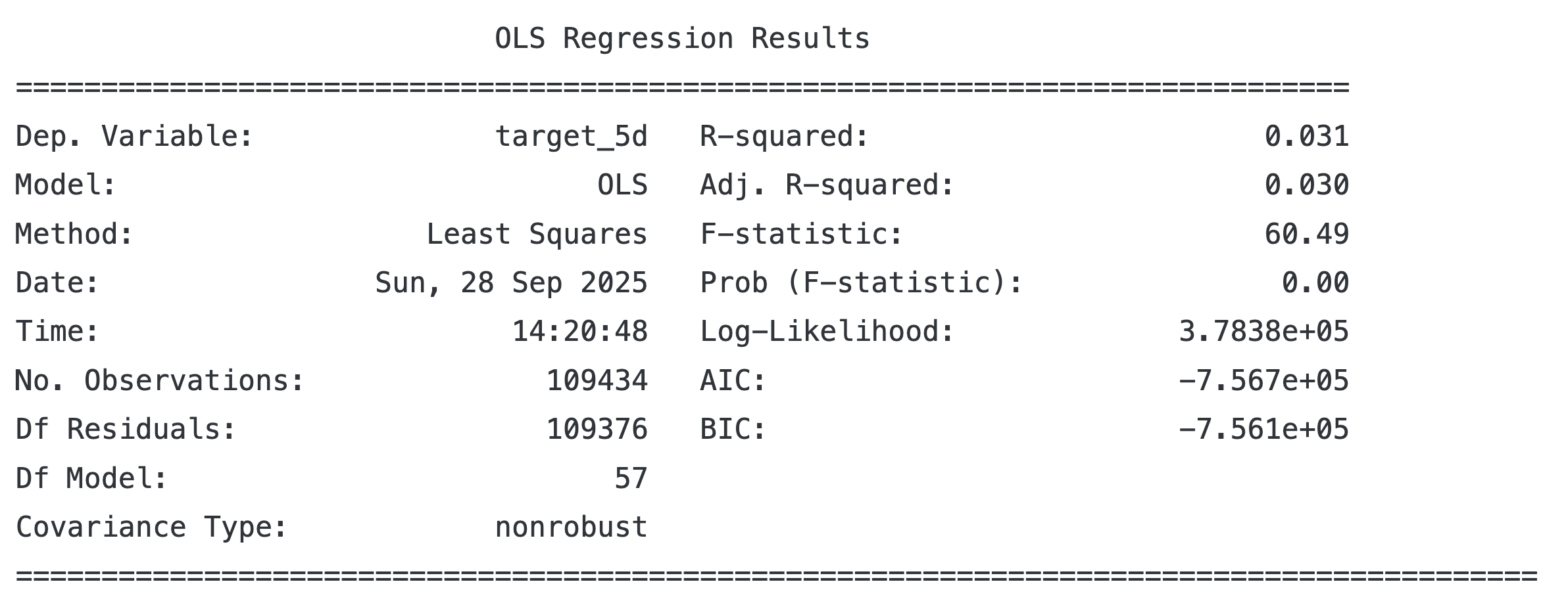
R方值比1-Day Returns要高一点
四、Obtain the residuals 计算残差
residuals analysis 残差分析
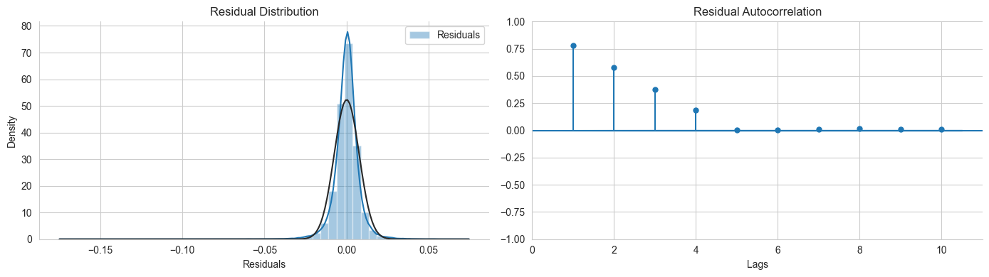
python
preds = trained_model.predict(add_constant(X))
residuals = y[target] - preds
fig, axes = plt.subplots(ncols=2, figsize=(14,4))
sns.distplot(residuals, fit=norm, ax=axes[0], axlabel='Residuals', label='Residuals')
axes[0].set_title('Residual Distribution')
axes[0].legend()
plot_acf(residuals, lags=10, zero=False, ax=axes[1], title='Residual Autocorrelation')
axes[1].set_xlabel('Lags')
sns.despine()
fig.tight_layout();
The residuals are normally distributed, it's good.
残差的分布是正态分布,这是好的。
But the autocorrelation is not good.
残差的自相关图不是很好(前几个Lags自相关系数在0.2以上),说明残差之间不是独立的。
10-Day Returns
python
target = 'target_10d'
model = OLS(endog=y[target], exog=add_constant(X))
trained_model = model.fit()
print(trained_model.summary())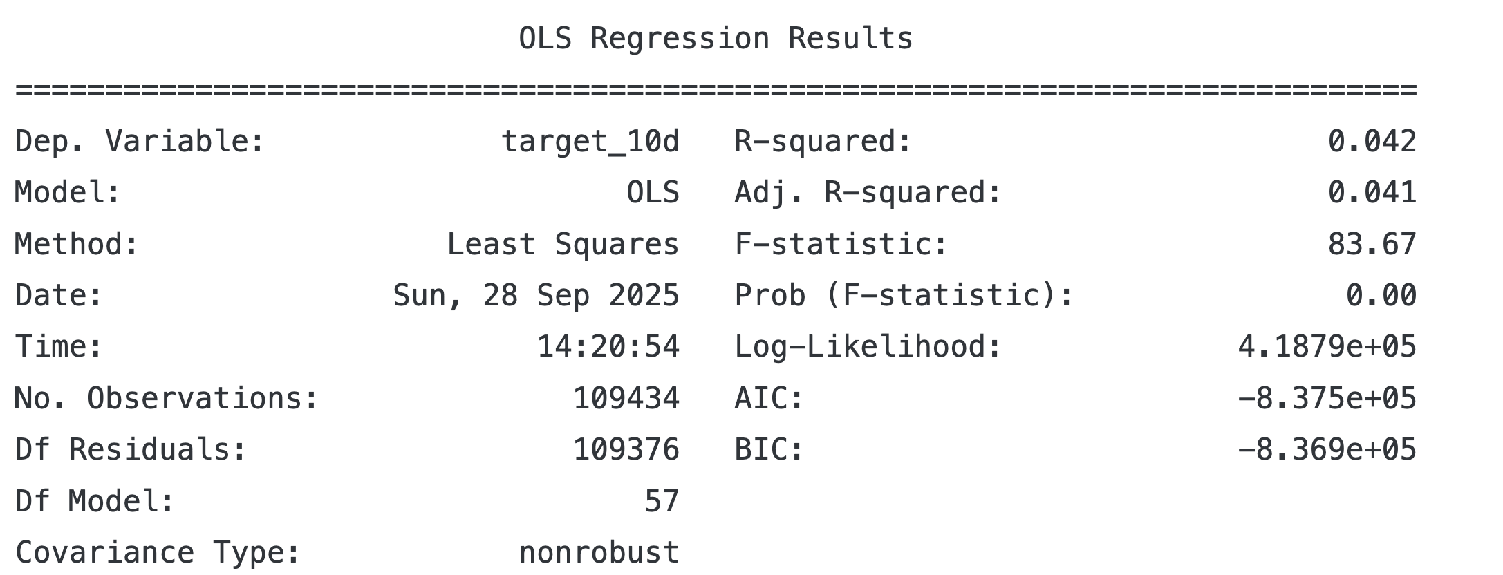
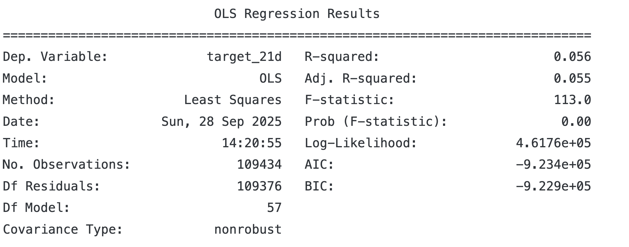
Monthly Returns
python
target = 'target_21d'
model = OLS(endog=y[target], exog=add_constant(X))
trained_model = model.fit()
print(trained_model.summary())