自己动手写深度学习框架（数值法实现神经网络的训练）

前面我们谈到了神经网络的基本原理。一个神经网络其实要运行起来，最主要的就是需要构建残差方程、计算梯度、梯度下降、合理化使用数据集这几个部分。在计算梯度这个部分，即使不会使用反向传播（bp）算法，也没有关系。使用数值法同样可以实现神经网络。下面就来看看，如果是用数值法，一般怎么实现神经网络。

0、基础头文件准备

如果不同函数位于不同文件，记得处理好import路径。

复制代码

import sys
import os
sys.path.append('../dataset')
sys.path.append('../common')
from mnist import *
from gradient import *
import numpy as np
import matplotlib.pyplot as plt

1、构建激励函数

激励函数是最基本的要求，这边直接生成即可，

复制代码

def sigmoid(x):
    return 1/(1 + np.exp(-x))

def softmax(x): 
    if x.ndim == 2: # should check dim of x
        x = x.T
        x = x - np.max(x, axis=0)
        y = np.exp(x) / np.sum(np.exp(x), axis=0)
        return y.T 

    x = x - np.max(x)
    return np.exp(x) / np.sum(np.exp(x))

2、创建损失函数

损失函数也是至关重要的，大家选一种自己擅长的损失函数即可，

复制代码

def cross_entropy_error(y,t):
    if y.ndim == 1:
        t = t.reshape(1, t.size)
        y = y.reshape(1, y.size)
    batch_size = y.shape[0]
    return -np.sum(t * np.log(y+1e-7))/batch_size  # process average batch error

3、构建神经网络

神经网络的构建，我们可以用一个类来完成。这个类里面，有参数的初始化、预测、损失函数计算、正确率计算和梯度向量计算。其中梯度向量计算最为重要，它本身又依赖于损失函数和预测函数。

复制代码

class TwoLayerNet:
    def __init__(self, input_size, hidden_size, output_size, weight_init_std=0.01):
        self.params={}
        self.params['W1'] = weight_init_std* np.random.randn(input_size, hidden_size)
        self.params['b1'] = np.zeros(hidden_size)
        self.params['W2'] = weight_init_std* np.random.randn(hidden_size, output_size)
        self.params['b2'] = np.zeros(output_size)

    def predict(self, x):
        W1,W2=self.params['W1'], self.params['W2']
        b1,b2=self.params['b1'], self.params['b2']

        a1 = np.dot(x,W1)+b1
        z1 = sigmoid(a1)
        a2 = np.dot(z1,W2)+b2
        y = softmax(a2)
        return y

    def loss(self, x, t):
        y = self.predict(x) # invoke predict function here
        return cross_entropy_error(y, t)

    def accuracy(self, x, t):
        y = self.predict(x)
        y = np.argmax(y, axis=1)
        t = np.argmax(t, axis=1)

        accuracy = np.sum(y==t)/float(x.shape[0])
        return accuracy

    def numerical_gradient(self, x, t):
        loss_W = lambda W: self.loss(x,t)# strange W defined, but not used in function

        grads={}
        grads['W1']=numerical_gradient(loss_W, self.params['W1']) # invoke global numberical_gradient function
        grads['b1']=numerical_gradient(loss_W, self.params['b1'])
        grads['W2']=numerical_gradient(loss_W, self.params['W2'])
        grads['b2']=numerical_gradient(loss_W, self.params['b2'])
        return grads

需要注意的是，梯度向量函数numerical_gradient函数当中，还使用到了全局梯度向量计算函数numerical_graident。所以这里不是递归运算，因为假设是递归运算的话，对应的函数应该写成self.numerical_gradient。

复制代码

def numerical_gradient(f, x):
    h = 1e-4 # 0.0001
    grad = np.zeros_like(x)
    
    it = np.nditer(x, flags=['multi_index'], op_flags=['readwrite'])
    while not it.finished:
        idx = it.multi_index
        tmp_val = x[idx]
        x[idx] = float(tmp_val) + h
        fxh1 = f(x) # f(x+h)
        
        x[idx] = tmp_val - h 
        fxh2 = f(x) # f(x-h)
        grad[idx] = (fxh1 - fxh2) / (2*h)
        
        x[idx] = tmp_val # restore
        it.iternext()   
        
    return grad

4、加载数据集，准备训练

数据集的准备也非常重要。开始学习的时候，一般都是采用公开训练集。等到后期实际使用的时候才会替换成客户的数据集，或者是自己用labelme标记的数据集。

复制代码

(x_train, t_train),(x_test, t_test) = load_mnist(normalize=True, one_hot_label=True)
train_loss_list=[]
train_acc_list=[]
test_acc_list=[]

iters_num=10000
train_size=x_train.shape[0]
batch_size=100 # 100 for each traning
learning_rate=0.1
network = TwoLayerNet(input_size=784, hidden_size=50, output_size=10)
iter_per_epoch=max(train_size/batch_size, 1)

5、用mini-batch的方法开始训练

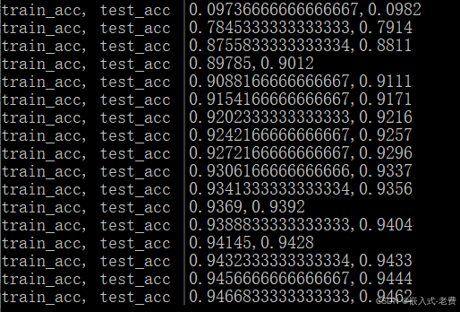
所谓的mini-batch，就是一次训练的时候，并不使用所有的数据集合，而是挑选若干个数据同时开始训练。**这样得到的参数梯度，其实是各个数据训练下，对应参数的平均值，这一点需要注意下。**训练的方法，一般就是用最经典的SGD对参数进行调优处理。经过一段时间训练后，一般会定时打印对应的正确率，也确认下是不是训练是有效的。

复制代码

for i in range(iters_num):
    batch_mask = np.random.choice(train_size, batch_size)
    x_batch = x_train[batch_mask] # 100*784
    t_batch = t_train[batch_mask] # 100*10

    grad = network.numerical_gradient(x_batch, t_batch)

    '''
    update parameter here
    '''

    for key in ('W1','b1','W2','b2'):
        network.params[key] -= learning_rate * grad[key]

    loss = network.loss(x_batch, t_batch)
    train_loss_list.append(loss)

    if i% iter_per_epoch == 0:
        train_acc = network.accuracy(x_train, t_train)
        test_acc = network.accuracy(x_test, t_test)
        train_acc_list.append(train_acc)
        test_acc_list.append(test_acc)
        print('train_acc, test_acc |' + str(train_acc) + ',' + str(test_acc))

6、实际绘图显示确认

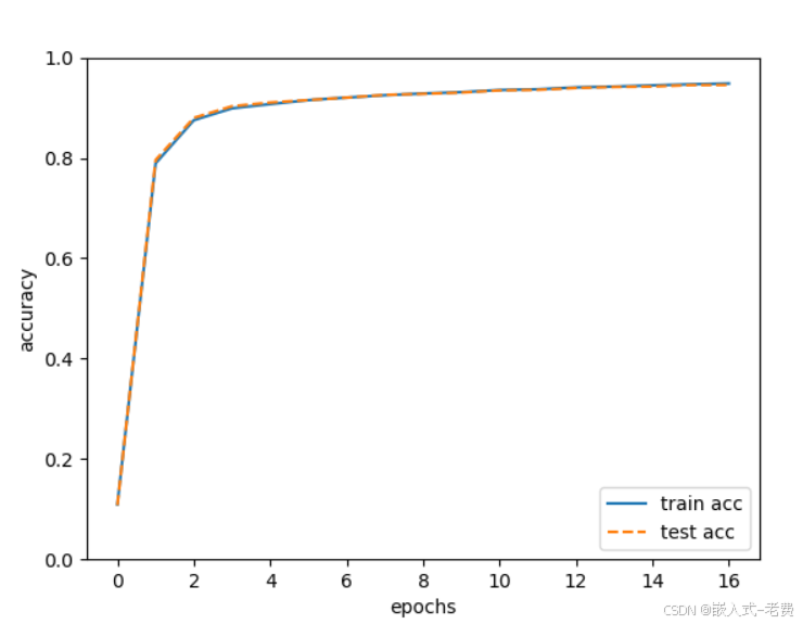
其实到这一步的时候，训练已经结束了，只是我们希望用matplotlib把对应的结果画出来而已。不画，也是可以的。只是画起来分析，效果会比较直观一点。

复制代码

markers = {'train': 'o', 'test': 's'}
x = np.arange(len(train_acc_list))
plt.plot(x, train_acc_list, label='train acc')
plt.plot(x, test_acc_list, label='test acc', linestyle='--')
plt.xlabel("epochs")
plt.ylabel("accuracy")
plt.ylim(0, 1.0)
plt.legend(loc='lower right')
plt.show()

7、实际训练

实际训练下来，大家会发现，这个思路是对的，但是效率是非常低的。差不多低两个数量级。如果大家没有概念的话，可以试想下，反向传播如果一个epoch，需要1s，那么数值法需要100s才能迭代一次。因此这种方法一般只是用来做交叉验证使用比较合适。

**不过从另外一个层面说，这是我们不借助tensorflow、pytorch、keras等第三方工具，第一次自己用python+numpy+matplotlib写一个简单的深度学习框架，本身学习的意义大于实际使用的意义。**它让我们知道训练本身是怎么一回事。毕竟相对来讲，forward预测还是好理解，反向训练要复杂一点。