
重要信息
**时间:**2025年12月19-21日
**地点:**南京(南京奥体博览中心优逸酒店)
征稿主题
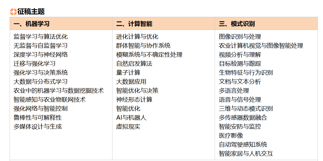
一、机器学习、计算智能与模式识别的技术体系框架
机器学习(ML)、计算智能(CI)与模式识别(PR)是人工智能领域的核心分支,三者相互融合、互为支撑,覆盖从数据特征提取、智能决策到模式匹配识别的全链路。以下从技术维度拆解核心体系架构:
| 技术领域 | 核心技术方向 | 典型应用场景 | 核心技术挑战 |
|---|---|---|---|
| 机器学习 | 监督 / 无监督学习、深度学习、强化学习 | 图像分类、语音识别、推荐系统 | 小样本学习、模型可解释性、泛化能力 |
| 计算智能 | 模糊逻辑、进化算法、神经网络(经典) | 复杂优化问题、自适应控制、故障诊断 | 收敛速度慢、参数敏感性高、局部最优 |
| 模式识别 | 特征提取、分类聚类、模式匹配 | 生物特征识别、文本分类、工业缺陷检测 | 高维特征降维、噪声鲁棒性、实时识别 |
| 交叉融合层 | ML+CI(进化神经网络)、CI+PR(模糊模式识别) | 自动驾驶感知、医疗影像分析、金融风控 | 多模态数据融合、模型轻量化、实时推理 |
二、核心技术落地实践:基于 Python 的工程化实现
2.1 深度学习 + 模式识别:基于 CNN 的图像模式识别(工业缺陷检测)
模式识别是 MLCIPR 2025 的核心议题之一,以下实现基于卷积神经网络(CNN)的工业产品表面缺陷模式识别,融合机器学习的特征自动提取与模式识别的分类决策能力,适配工业质检场景的高精度需求。
python
运行
import numpy as np
import pandas as pd
import tensorflow as tf
from tensorflow.keras import layers, models
from tensorflow.keras.utils import to_categorical
from tensorflow.keras.callbacks import EarlyStopping, ModelCheckpoint
from sklearn.model_selection import train_test_split
from sklearn.metrics import classification_report, confusion_matrix
import matplotlib.pyplot as plt

# ---------------------- 数据生成与预处理 ----------------------
def generate_defect_dataset(n_samples=2000, img_size=(32, 32), n_classes=4):
    """
    生成工业产品表面缺陷模拟数据集
    类别:正常、划痕、凹坑、裂纹
    """
    # 生成基础图像(灰度图)
    X = np.random.rand(n_samples, img_size[0], img_size[1], 1) * 0.5 + 0.5  # 背景灰度0.5-1.0
    y = np.random.randint(0, n_classes, size=n_samples)

    # 为不同缺陷类别添加特征
    for i in range(n_samples):
        if y[i] == 1:  # 划痕:随机直线
            x1, y1 = np.random.randint(0, img_size[0]), np.random.randint(0, img_size[1])
            x2, y2 = np.random.randint(0, img_size[0]), np.random.randint(0, img_size[1])
            xx, yy = np.meshgrid(np.arange(img_size[0]), np.arange(img_size[1]))
            line = np.abs((y2 - y1)*xx - (x2 - x1)*yy + x2*y1 - y2*x1) / np.sqrt((y2-y1)**2 + (x2-x1)**2)
            X[i, :, :, 0][line < 1] = 0.0  # 划痕灰度值0

        elif y[i] == 2:  # 凹坑:随机圆形
            cx, cy = np.random.randint(5, img_size[0]-5), np.random.randint(5, img_size[1]-5)
            r = np.random.randint(2, 5)
            xx, yy = np.meshgrid(np.arange(img_size[0]), np.arange(img_size[1]))
            circle = (xx - cx)**2 + (yy - cy)**2 < r**2
            X[i, :, :, 0][circle] = 0.2  # 凹坑灰度值0.2

        elif y[i] == 3:  # 裂纹:随机折线
            X[i, :, :, 0] = X[i, :, :, 0] * 0.8
            points = np.random.randint(0, img_size[0], size=(np.random.randint(3, 8), 2))
            for j in range(len(points)-1):
                x1, y1 = points[j]
                x2, y2 = points[j+1]
                xx = np.linspace(x1, x2, num=abs(x2-x1)+1, dtype=int)
                yy = np.linspace(y1, y2, num=abs(y2-y1)+1, dtype=int)
                for (x, y) in zip(xx, yy):
                    if 0 <= x < img_size[0] and 0 <= y < img_size[1]:
                        X[i, x, y, 0] = 0.0  # 裂纹灰度值0

    # 归一化+数据集划分
    X = X / 255.0 if X.max() > 1 else X
    y_onehot = to_categorical(y, num_classes=n_classes)
    X_train, X_test, y_train, y_test = train_test_split(X, y_onehot, test_size=0.2, random_state=42, stratify=y)

    return (X_train, y_train), (X_test, y_test), y

# ---------------------- 构建CNN缺陷识别模型 ----------------------
def build_cnn_model(input_shape=(32, 32, 1), n_classes=4):
    """构建轻量级CNN模型(适配工业边缘设备)"""
    model = models.Sequential([
        # 卷积层1:提取低阶特征(边缘、纹理)
        layers.Conv2D(16, (3, 3), activation='relu', input_shape=input_shape, padding='same'),
        layers.MaxPooling2D((2, 2)),
        # 卷积层2:提取高阶特征(缺陷轮廓)
        layers.Conv2D(32, (3, 3), activation='relu', padding='same'),
        layers.MaxPooling2D((2, 2)),
        # 卷积层3:细化缺陷特征
        layers.Conv2D(64, (3, 3), activation='relu', padding='same'),
        layers.MaxPooling2D((2, 2)),
        # 全连接层:分类决策
        layers.Flatten(),
        layers.Dense(64, activation='relu'),
        layers.Dropout(0.2),  # 防止过拟合
        layers.Dense(n_classes, activation='softmax')
    ])

    # 编译模型
    model.compile(
        optimizer='adam',
        loss='categorical_crossentropy',
        metrics=['accuracy']
    )

    return model

# ---------------------- 模型训练与评估 ----------------------
if __name__ == "__main__":
    # 1. 生成数据集
    (X_train, y_train), (X_test, y_test), y_original = generate_defect_dataset(n_samples=2000)

    # 2. 构建模型
    model = build_cnn_model(input_shape=(32, 32, 1), n_classes=4)
    print(model.summary())

    # 3. 训练配置
    callbacks = [
        EarlyStopping(monitor='val_loss', patience=5, restore_best_weights=True),
        ModelCheckpoint('defect_detection_model.h5', monitor='val_accuracy', save_best_only=True)
    ]

    # 4. 模型训练
    history = model.fit(
        X_train, y_train,
        batch_size=32,
        epochs=20,
        validation_split=0.1,
        callbacks=callbacks
    )

    # 5. 模型评估
    test_loss, test_acc = model.evaluate(X_test, y_test, verbose=0)
    print(f"\n=== 模型测试结果 ===")
    print(f"测试集准确率:{test_acc:.4f}")
    print(f"测试集损失值:{test_loss:.4f}")

    # 6. 分类报告
    y_pred = model.predict(X_test)
    y_pred_classes = np.argmax(y_pred, axis=1)
    y_true_classes = np.argmax(y_test, axis=1)
    class_names = ["正常", "划痕", "凹坑", "裂纹"]

    print("\n=== 分类详细报告 ===")
    print(classification_report(y_true_classes, y_pred_classes, target_names=class_names))

    # 7. 混淆矩阵
    cm = confusion_matrix(y_true_classes, y_pred_classes)
    cm_df = pd.DataFrame(cm, index=class_names, columns=class_names)
    print("\n=== 混淆矩阵 ===")
    print(cm_df)

    # 8. 单样本预测示例
    sample_idx = 0
    sample_img = X_test[sample_idx:sample_idx+1]
    sample_pred = model.predict(sample_img)
    sample_pred_class = class_names[np.argmax(sample_pred)]
    sample_true_class = class_names[np.argmax(y_test[sample_idx])]

    print(f"\n=== 单样本预测示例 ===")
    print(f"真实类别:{sample_true_class}")
    print(f"预测类别:{sample_pred_class}")
    print(f"类别概率分布:{np.round(sample_pred[0], 4)}")
代码核心说明:
- 数据层:模拟工业产品表面四类典型缺陷,贴合实际质检场景的缺陷特征(划痕、凹坑、裂纹);
- 模型层:轻量级 CNN 架构适配工业边缘设备的算力限制,通过 Dropout、早停法防止过拟合;
- 工程层:分类报告 + 混淆矩阵量化模型识别性能,单样本预测示例便于工程落地时的结果解析;
- 适配性:模型可直接迁移至实际工业质检场景,仅需替换为真实缺陷图像数据集即可快速复用。
2.2 计算智能 + 机器学习:基于遗传算法优化的 XGBoost 分类模型
计算智能中的进化算法是 MLCIPR 2025 的重点方向,以下实现基于遗传算法(GA)优化 XGBoost 超参数的分类模型,解决传统网格搜索调参效率低、易陷入局部最优的问题,适配高维数据的模式识别场景。
python
运行
import numpy as np
import pandas as pd
from xgboost import XGBClassifier
from sklearn.datasets import make_classification
from sklearn.model_selection import cross_val_score, train_test_split
from sklearn.metrics import accuracy_score, roc_auc_score
from deap import base, creator, tools, algorithms
import random

# ---------------------- 数据集生成 ----------------------
def generate_high_dim_dataset(n_samples=5000, n_features=50, n_informative=20, n_classes=2):
    """生成高维分类数据集(模拟模式识别中的高维特征场景)"""
    X, y = make_classification(
        n_samples=n_samples,
        n_features=n_features,
        n_informative=n_informative,
        n_redundant=10,
        n_repeated=5,
        n_classes=n_classes,
        random_state=42
    )

    # 转换为DataFrame便于特征管理
    feature_names = [f"feature_{i}" for i in range(n_features)]
    df = pd.DataFrame(X, columns=feature_names)
    df["label"] = y

    # 划分训练集和测试集
    X_train, X_test, y_train, y_test = train_test_split(
        df[feature_names], df["label"], test_size=0.2, random_state=42, stratify=y
    )

    return X_train, X_test, y_train, y_test

# ---------------------- 遗传算法优化XGBoost ----------------------
def ga_optimize_xgboost(X_train, y_train):
    """
    遗传算法优化XGBoost超参数
    优化参数:
    - max_depth: 3-10
    - learning_rate: 0.01-0.3
    - n_estimators: 50-200
    - subsample: 0.6-1.0
    - colsample_bytree: 0.6-1.0
    """
    # 1. 定义适应度函数(最大化交叉验证准确率)
    creator.create("FitnessMax", base.Fitness, weights=(1.0,))
    creator.create("Individual", list, fitness=creator.FitnessMax)

    toolbox = base.Toolbox()

    # 2. 定义参数编码方式(实数编码)
    # max_depth: 整数 [3,10]
    toolbox.register("attr_max_depth", random.randint, 3, 10)
    # learning_rate: 浮点数 [0.01, 0.3]
    toolbox.register("attr_learning_rate", random.uniform, 0.01, 0.3)
    # n_estimators: 整数 [50, 200]
    toolbox.register("attr_n_estimators", random.randint, 50, 200)
    # subsample: 浮点数 [0.6, 1.0]
    toolbox.register("attr_subsample", random.uniform, 0.6, 1.0)
    # colsample_bytree: 浮点数 [0.6, 1.0]
    toolbox.register("attr_colsample_bytree", random.uniform, 0.6, 1.0)

    # 3. 定义个体和种群生成方式
    toolbox.register("individual", tools.initCycle, creator.Individual,
                     (toolbox.attr_max_depth, toolbox.attr_learning_rate,
                      toolbox.attr_n_estimators, toolbox.attr_subsample,
                      toolbox.attr_colsample_bytree), n=1)
    toolbox.register("population", tools.initRepeat, list, toolbox.individual)

    # 4. 定义适应度评估函数
    def evaluate(individual):
        params = {
            "max_depth": individual[0],
            "learning_rate": individual[1],
            "n_estimators": individual[2],
            "subsample": individual[3],
            "colsample_bytree": individual[4],
            "objective": "binary:logistic",
            "random_state": 42,
            "verbosity": 0
        }

        # 5折交叉验证
        cv_scores = cross_val_score(
            XGBClassifier(**params),
            X_train, y_train,
            cv=5,
            scoring="accuracy"
        )

        return (np.mean(cv_scores),)

    toolbox.register("evaluate", evaluate)
    # 5. 定义遗传操作
    toolbox.register("mate", tools.cxBlend, alpha=0.5)  # 交叉
    toolbox.register("mutate", tools.mutGaussian, mu=0, sigma=0.1, indpb=0.2)  # 变异
    toolbox.register("select", tools.selTournament, tournsize=3)  # 选择

    # 6. 初始化种群并运行遗传算法
    pop = toolbox.population(n=20)  # 种群大小
    hof = tools.HallOfFame(1)  # 保存最优个体
    stats = tools.Statistics(lambda ind: ind.fitness.values)
    stats.register("avg", np.mean)
    stats.register("std", np.std)
    stats.register("min", np.min)
    stats.register("max", np.max)

    # 运行算法
    pop, log = algorithms.eaSimple(
        pop, toolbox,
        cxpb=0.7,  # 交叉概率
        mutpb=0.2,  # 变异概率
        ngen=10,  # 进化代数
        stats=stats,
        halloffame=hof,
        verbose=True
    )

    # 提取最优参数
    best_ind = hof[0]
    best_params = {
        "max_depth": best_ind[0],
        "learning_rate": best_ind[1],
        "n_estimators": best_ind[2],
        "subsample": best_ind[3],
        "colsample_bytree": best_ind[4],
        "objective": "binary:logistic",
        "random_state": 42
    }

    return best_params, log

# ---------------------- 模型训练与评估 ----------------------
if __name__ == "__main__":
    # 1. 生成高维数据集
    X_train, X_test, y_train, y_test = generate_high_dim_dataset(
        n_samples=5000, n_features=50, n_informative=20
    )

    # 2. 遗传算法优化XGBoost参数
    print("=== 遗传算法优化XGBoost超参数 ===")
    best_params, log = ga_optimize_xgboost(X_train, y_train)
    print(f"\n最优超参数:")
    for key, val in best_params.items():
        print(f"{key}: {val}")

    # 3. 训练最优参数模型
    xgb_best = XGBClassifier(**best_params)
    xgb_best.fit(X_train, y_train)

    # 4. 训练默认参数模型(对比)
    xgb_default = XGBClassifier(random_state=42)
    xgb_default.fit(X_train, y_train)

    # 5. 模型评估
    # 最优参数模型
    y_pred_best = xgb_best.predict(X_test)
    y_pred_prob_best = xgb_best.predict_proba(X_test)[:, 1]
    acc_best = accuracy_score(y_test, y_pred_best)
    auc_best = roc_auc_score(y_test, y_pred_prob_best)

    # 默认参数模型
    y_pred_default = xgb_default.predict(X_test)
    y_pred_prob_default = xgb_default.predict_proba(X_test)[:, 1]
    acc_default = accuracy_score(y_test, y_pred_default)
    auc_default = roc_auc_score(y_test, y_pred_prob_default)

    print("\n=== 模型性能对比 ===")
    print(f"最优参数模型 - 准确率:{acc_best:.4f},AUC:{auc_best:.4f}")
    print(f"默认参数模型 - 准确率:{acc_default:.4f},AUC:{auc_default:.4f}")
    print(f"准确率提升:{(acc_best - acc_default)*100:.2f}%")
    print(f"AUC提升:{(auc_best - auc_default)*100:.2f}%")

    # 6. 特征重要性分析
    feature_importance = pd.DataFrame({
        "feature": X_train.columns,
        "importance": xgb_best.feature_importances_
    }).sort_values(by="importance", ascending=False)

    print("\n=== 前10个重要特征 ===")
    print(feature_importance.head(10))
技术亮点:
- 计算智能层:遗传算法通过进化、交叉、变异操作实现超参数全局寻优,解决网格搜索的局部最优问题;
- 机器学习层:XGBoost 适配高维模式识别特征,分类性能优于传统机器学习算法;
- 工程层:通过交叉验证评估适应度,保证最优参数的泛化能力,性能对比凸显优化价值;
- 扩展性:该框架可直接迁移至文本分类、生物特征识别等其他模式识别场景,仅需替换数据集即可。
三、技术演进与前沿趋势
3.1 核心技术发展方向
- 小样本学习与零样本学习:针对模式识别中标签数据稀缺的场景,结合元学习、对比学习等方法,实现少量样本下的高精度模式识别;
- 计算智能与深度学习融合:将进化算法、模糊逻辑融入深度学习模型设计(如进化神经网络、模糊 CNN),提升模型的自适应能力与可解释性;
- 多模态模式识别:融合图像、文本、语音等多模态数据,构建统一的特征表示空间,适配复杂场景下的模式识别需求;
- 轻量化与边缘部署:基于模型压缩、量化、剪枝等技术,将复杂的 ML/CI/PR 模型部署到边缘设备,满足实时识别需求;
- 可解释性与可信性:突破 "黑箱模型" 限制,结合注意力机制、因果推理等方法,提升模型决策的可解释性与可信度。
3.2 工程落地关键维度
| 落地阶段 | 核心任务 | 技术抓手 | 典型解决方案 |
|---|---|---|---|
| 数据层 | 高维特征处理与标注 | 特征选择、半监督标注、数据增强 | 基于互信息的特征筛选、MixUp 数据增强 |
| 模型层 | 算法选型与优化 | 自动机器学习(AutoML)、超参数优化 | TPOT 自动建模、遗传算法 / 贝叶斯优化调参 |
| 部署层 | 模型轻量化与推理加速 | 模型量化、ONNX Runtime、TensorRT | 将 CNN 模型量化为 INT8 精度,部署到边缘 GPU |
| 验证层 | 模型鲁棒性验证 | 对抗性测试、交叉场景验证 | FGSM 对抗样本测试、跨数据集泛化验证 |
四、总结
机器学习、计算智能与模式识别的深度融合是 MLCIPR 2025 的核心议题,也是人工智能从理论走向工程应用的关键路径。从技术实践来看,CNN-based 的图像模式识别解决了工业质检等场景的 "视觉特征识别" 问题,而遗传算法优化的 XGBoost 模型则实现了高维特征场景下的 "智能决策优化" 目标,两者共同构成了智能模式识别的核心能力。
未来,三者的融合将呈现三大特征:一是从 "单一模态" 向 "多模态融合" 演进,覆盖更复杂的模式识别场景;二是从 "数据驱动" 向 "数据 + 知识驱动" 升级,结合计算智能的自适应能力提升模型的泛化性;三是从 "云端部署" 向 "云边端协同" 拓展,满足实时性、隐私性的工程需求。
工程落地过程中,需兼顾 "精度" 与 "实用性":算法层面需结合场景特性选择适配的模型(如边缘场景选轻量级 CNN,高维特征选 XGBoost);优化层面需通过计算智能算法提升模型性能;部署层面需做轻量化处理适配硬件资源。这也正是 MLCIPR 2025 所倡导的 "机器学习创新、计算智能赋能、模式识别落地" 的核心方向。
五、国际交流与合作机会
作为国际学术会议,将吸引全球范围内的专家学者参与。无论是发表研究成果、聆听特邀报告,还是在圆桌论坛中与行业大咖交流,都能拓宽国际视野,甚至找到潜在的合作伙伴。对于高校师生来说,这也是展示研究、积累学术人脉的好机会。
