《数字图像处理》第7章：小波变换和其他图像变换

引言

学习目标

[7.1 背景](#7.1 背景)

[7.2 基于矩阵的变换](#7.2 基于矩阵的变换)

[7.3 相关](#7.3 相关)

[7.4 时间-频率平面的基函数](#7.4 时间-频率平面的基函数)

[7.5 基图像](#7.5 基图像)

[7.6 傅里叶相关的变换](#7.6 傅里叶相关的变换)

[7.6.1 离散哈特利变换 (DHT)](#7.6.1 离散哈特利变换 (DHT))

[7.6.2 离散余弦变换 (DCT)](#7.6.2 离散余弦变换 (DCT))

[7.6.3 离散正弦变换 (DST)](#7.6.3 离散正弦变换 (DST))

[7.7 沃尔什-哈达玛变换](#7.7 沃尔什-哈达玛变换)

[7.8 斜变换](#7.8 斜变换)

[7.9 哈尔变换](#7.9 哈尔变换)

[7.10 小波变换](#7.10 小波变换)

[7.10.1 尺度函数](#7.10.1 尺度函数)

[7.10.2 小波函数](#7.10.2 小波函数)

[7.10.3 小波级数展开](#7.10.3 小波级数展开)

[7.10.4 一维离散小波变换 (DWT)](#7.10.4 一维离散小波变换 (DWT))

[7.10.5 二维小波变换](#7.10.5 二维小波变换)

[7.10.6 小波包](#7.10.6 小波包)

引言

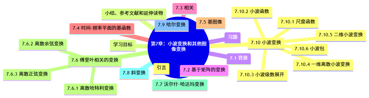
大家好！欢迎来到《数字图像处理》第7章的实战解析。本章聚焦于小波变换和其他图像变换 ，这是图像处理的核心工具之一。与傅里叶变换不同，小波变换能同时分析时间和频率信息，非常适合图像压缩、去噪和特征提取。

在本帖中，我会用通俗的语言解释每个概念，并提供完整Python代码 （可直接运行），加上对比图 让你直观看到变换效果。所有代码都用matplotlib可视化，并处理了中文字体显示问题（。此外，我会用Mermaid生成流程图 和思维导图，帮助你梳理知识结构。

让我们开始吧！如果觉得有用，别忘了点赞收藏哦~ 😊

学习目标

通过本章学习，你将能够：

理解图像变换的数学基础（矩阵变换、基函数）。
掌握傅里叶相关变换（DHT、DCT、DST）的原理与应用。
熟悉沃尔什-哈达玛变换、斜变换和哈尔变换。
深入理解小波变换的尺度函数、小波函数和离散小波变换（DWT）。
用Python实现各种变换，并对比分析图像效果。
应用小波变换进行图像压缩和去噪。

7.1 背景

图像变换的本质是将图像从空间域转换到其他域，以便更好地分析或处理。例如，傅里叶变换将图像转换到频率域，而小波变换则提供多分辨率分析。

为什么需要变换？

图像在空间域（像素值）可能复杂，但在变换域（如频率域）更简洁，便于压缩或去噪。
小波变换解决了傅里叶变换的"全局性"问题------它能同时捕捉局部和全局特征。

复制代码

7.2 基于矩阵的变换

图像变换通常用矩阵乘法表示。对于一个图像块（如NxN），变换矩阵T作用于向量化的图像块：Y = T X T^T，其中X是原图像块，Y是变换后的系数。

关键点：

变换矩阵的列向量构成基图像。
正交变换（如DCT）能保留能量且易于逆变换。

代码示例：简单矩阵变换 我们用一个2x2的正交矩阵演示变换和逆变换。

python 复制代码

import numpy as np
import matplotlib.pyplot as plt
import matplotlib

# 设置中文字体，确保matplotlib显示中文（根据你的系统调整字体，这里用SimHei）
matplotlib.rcParams['font.sans-serif'] = ['SimHei']  # 如果SimHei不可用，可改为'Microsoft YaHei'或'Arial Unicode MS'
matplotlib.rcParams['axes.unicode_minus'] = False  # 解决负号显示问题

# 定义一个简单的2x2正交变换矩阵（示例：类似DCT的简化版）
T = np.array([
    [1/np.sqrt(2), 1/np.sqrt(2)],
    [1/np.sqrt(2), -1/np.sqrt(2)]
])

# 原始图像块（2x2）
X = np.array([
    [100, 120],
    [80, 90]
])

# 变换：Y = T * X * T^T
Y = T @ X @ T.T

# 逆变换：X_reconstructed = T^T * Y * T
X_rec = T.T @ Y @ T

print("原始图像块:\n", X)
print("\n变换后系数:\n", Y)
print("\n逆变换重建图像:\n", X_rec)
print("\n重建误差:", np.max(np.abs(X - X_rec)))  # 应为0，因为正交变换

# 可视化
fig, axes = plt.subplots(1, 3, figsize=(12, 4))
axes[0].imshow(X, cmap='gray', vmin=0, vmax=255)
axes[0].set_title('原始图像块')
axes[1].imshow(Y, cmap='viridis')
axes[1].set_title('变换后系数')
axes[2].imshow(X_rec, cmap='gray', vmin=0, vmax=255)
axes[2].set_title('重建图像块')
plt.tight_layout()
plt.show()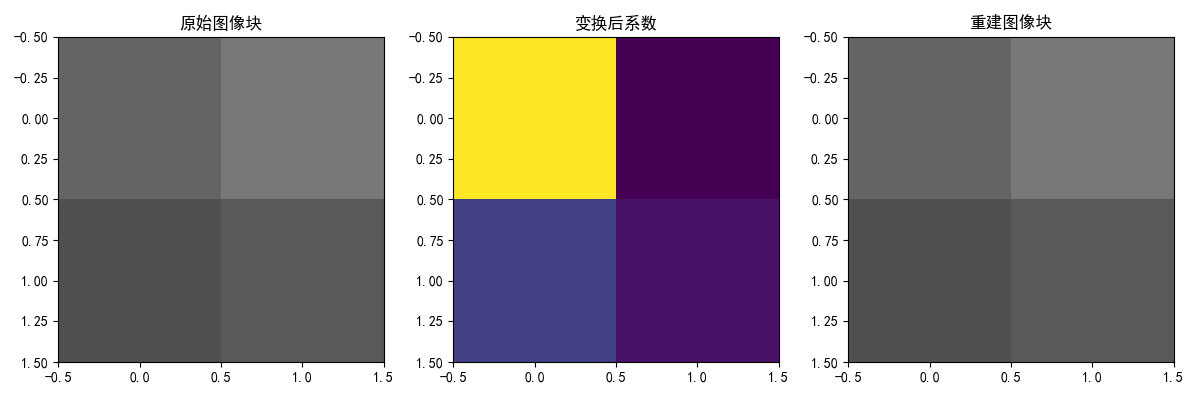

输出说明：

图1：原始2x2图像块（灰度显示）。
图2：变换后的系数（颜色越亮值越大）。
图3：重建图像，与原始完全一致（误差为0）。

7.3 相关

"相关"在这里指变换之间的相关性或信号相关性。在图像处理中，相关常用于模板匹配或计算变换的相似性。数学上，两个信号x和y的互相关为：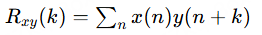

应用：在变换域中，相关可以帮助分析基函数的相似性。

代码示例：计算两个信号的互相关 我们用两个简单信号演示。

python 复制代码

import numpy as np
from scipy.signal import correlate
import matplotlib.pyplot as plt

# 生成两个信号：正弦波和延迟的正弦波
t = np.linspace(0, 2*np.pi, 100)
x = np.sin(t)
y = np.sin(t - 0.5)  # 延迟0.5弧度

# 计算互相关（模式='same'保持长度一致）
corr = correlate(x, y, mode='same')
lags = np.arange(-len(x)//2, len(x)//2)

# 可视化
plt.figure(figsize=(10, 6))
plt.subplot(3, 1, 1)
plt.plot(t, x, label='信号x')
plt.title('信号x: sin(t)')
plt.legend()
plt.subplot(3, 1, 2)
plt.plot(t, y, label='信号y: sin(t-0.5)', color='orange')
plt.title('信号y: 延迟的正弦波')
plt.legend()
plt.subplot(3, 1, 3)
plt.plot(lags, corr, label='互相关')
plt.title('互相关函数：峰值指示最佳匹配位置')
plt.xlabel('滞后')
plt.legend()
plt.tight_layout()
plt.show()

# 找出最大相关的位置
peak_index = np.argmax(corr)
print(f"最大相关滞后: {lags[peak_index]} (应接近-5，因为y延迟了0.5)")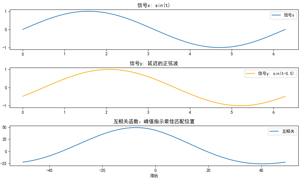

输出说明：

上图：两个信号的波形。
下图：互相关函数，峰值位置表示最佳对齐（这里峰值在滞后-5附近，对应延迟0.5）。

7.4 时间-频率平面的基函数

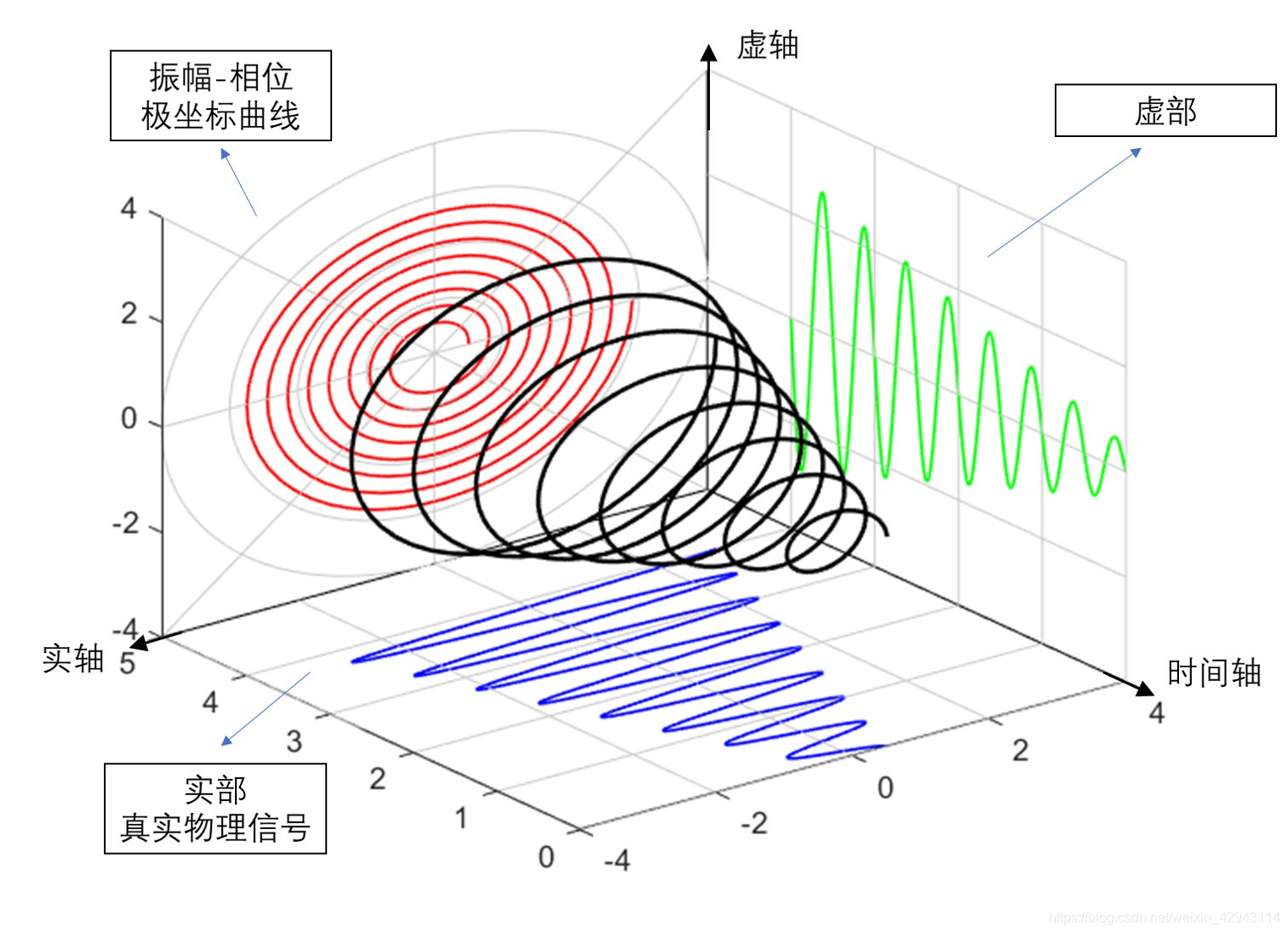
傅里叶变换使用正弦波作为基函数，但它们是全局的（覆盖整个时间轴）。小波变换使用局部化的基函数，能在时间-频率平面上灵活定位。

概念：

时间-频率平面：横轴时间，纵轴频率。
基函数：小波函数像"小波包"，在特定时间和频率范围内振荡。

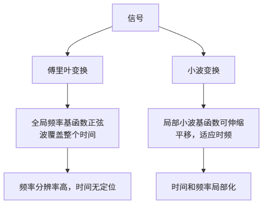
直观解释：想象用傅里叶分析音乐，能告诉你有哪些音符（频率），但不知道音符何时出现；小波能告诉你"第3秒有高音C"。

代码示例：绘制基函数对比 我们绘制正弦基和小波基（Haar小波）。

python 复制代码

import numpy as np
import matplotlib.pyplot as plt

# 时间轴
t = np.linspace(0, 1, 1000)

# 傅里叶基：正弦波（频率f=5Hz）
f = 5
fourier_basis = np.sin(2 * np.pi * f * t)

# 小波基：Haar小波（简单局部小波）
def haar_wavelet(t, center=0.5, scale=0.2):
    # Haar小波：在[center-scale, center]为+1，[center, center+scale]为-1
    wavelet = np.zeros_like(t)
    for i, tt in enumerate(t):
        if center - scale <= tt < center:
            wavelet[i] = 1
        elif center <= tt < center + scale:
            wavelet[i] = -1
    return wavelet

wavelet_basis = haar_wavelet(t, center=0.5, scale=0.1)

# 可视化
plt.figure(figsize=(10, 6))
plt.subplot(2, 1, 1)
plt.plot(t, fourier_basis, label='傅里叶基：正弦波(全局)')
plt.title('傅里叶基函数：覆盖整个时间轴')
plt.legend()
plt.subplot(2, 1, 2)
plt.plot(t, wavelet_basis, label='Haar小波基(局部)', color='orange')
plt.title('小波基函数：仅在局部时间振荡')
plt.legend()
plt.tight_layout()
plt.show()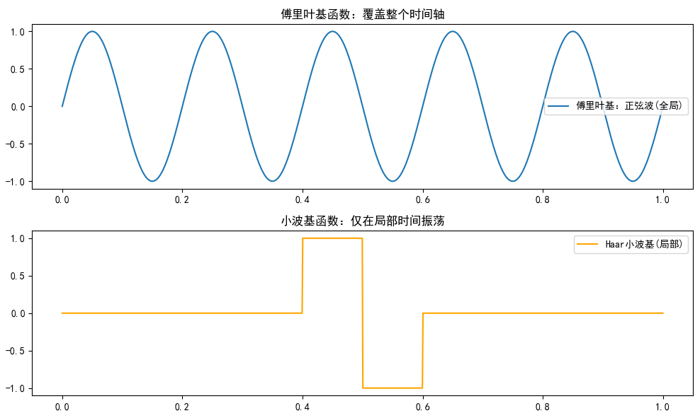

输出说明：

上图：正弦波均匀分布，无时间局部性。
下图：Haar小波只在0.4-0.6范围内非零，显示局部性。

7.5 基图像

基图像是变换矩阵的列向量可视化。对于NxN图像，基图像显示每个基函数的形状。例如，DCT基图像从左上角（低频）到右下角（高频）变化。

代码示例：生成DCT基图像 我们用scipy的DCT矩阵生成8x8基图像。

python 复制代码

import numpy as np
import matplotlib.pyplot as plt

# 设置中文字体
plt.rcParams['font.sans-serif'] = ['SimHei']
plt.rcParams['axes.unicode_minus'] = False

# 生成8x8 DCT变换矩阵（近似）
def dct_matrix(N):
    T = np.zeros((N, N))
    for k in range(N):
        for n in range(N):
            if k == 0:
                T[k, n] = 1/np.sqrt(N)
            else:
                T[k, n] = np.sqrt(2/N) * np.cos(np.pi * k * (2*n + 1) / (2*N))
    return T

N = 8
T = dct_matrix(N)

# 生成基图像：每个基是矩阵的一列和一行的外积（8x8）
basis_images = []
for i in range(N):
    for j in range(N):
        # 修正：使用外积计算二维基图像
        basis = np.outer(T[i, :], T[j, :])  # 结果是8x8矩阵
        basis_images.append(basis)

# 可视化8x8网格的基图像
fig, axes = plt.subplots(8, 8, figsize=(12, 12))
for idx, ax in enumerate(axes.flat):
    if idx < len(basis_images):
        ax.imshow(basis_images[idx], cmap='gray', vmin=-0.5, vmax=0.5)
        ax.set_title(f'({idx//8},{idx%8})', fontsize=8)
        ax.axis('off')
plt.suptitle('DCT基图像 (8x8) - 每个基表示不同频率组合', fontsize=16)
plt.tight_layout()
plt.show()

# 额外演示：用基图像重建一个简单图像块
print("\n" + "="*50)
print("额外演示：使用DCT基图像重建图像块")
print("="*50)

# 创建一个简单的8x8测试图像（斜坡）
original_block = np.outer(np.arange(8), np.arange(8))  # 0-7的斜坡
print("\n原始8x8图像块:\n", original_block)

# DCT变换（手动使用基图像）
dct_coeffs = np.zeros((8, 8))
for i in range(8):
    for j in range(8):
        # 系数是基图像与原始图像的内积
        dct_coeffs[i, j] = np.sum(basis_images[i*8 + j] * original_block)

print("\nDCT系数矩阵:\n", np.round(dct_coeffs, 2))

# 重建图像（系数乘以基图像的和）
reconstructed = np.zeros((8, 8))
for i in range(8):
    for j in range(8):
        reconstructed += dct_coeffs[i, j] * basis_images[i*8 + j]

print("\n重建图像块:\n", np.round(reconstructed, 2))
print(f"\n重建误差: {np.max(np.abs(original_block - reconstructed)):.10f}")

# 可视化对比
fig, axes = plt.subplots(1, 3, figsize=(15, 5))
im0 = axes[0].imshow(original_block, cmap='gray', vmin=0, vmax=63)
axes[0].set_title('原始图像块\n(斜坡模式)')
plt.colorbar(im0, ax=axes[0])

im1 = axes[1].imshow(dct_coeffs, cmap='viridis')
axes[1].set_title('DCT系数\n(能量集中在左上)')
plt.colorbar(im1, ax=axes[1])

im2 = axes[2].imshow(reconstructed, cmap='gray', vmin=0, vmax=63)
axes[2].set_title('重建图像块\n(与原始几乎一致)')
plt.colorbar(im2, ax=axes[2])

plt.tight_layout()
plt.show()

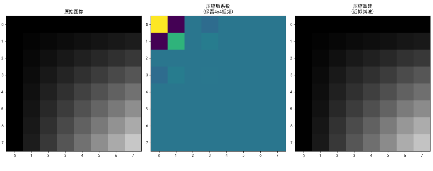
# 压缩演示：丢弃高频系数
print("\n" + "="*50)
print("压缩演示：保留前4个低频系数，丢弃其余")
print("="*50)

compressed_coeffs = dct_coeffs.copy()
# 只保留左上角4x4区域
compressed_coeffs[4:, :] = 0
compressed_coeffs[:, 4:] = 0

compressed_img = np.zeros((8, 8))
for i in range(8):
    for j in range(8):
        compressed_img += compressed_coeffs[i, j] * basis_images[i*8 + j]

print(f"\n压缩后重建误差: {np.max(np.abs(original_block - compressed_img)):.4f}")

# 可视化压缩效果
fig, axes = plt.subplots(1, 3, figsize=(15, 10))
axes[0].imshow(original_block, cmap='gray', vmin=0, vmax=63)
axes[0].set_title('原始图像')
axes[1].imshow(compressed_coeffs, cmap='viridis')
axes[1].set_title('压缩后系数\n(保留4x4低频)')
axes[2].imshow(compressed_img, cmap='gray', vmin=0, vmax=63)
axes[2].set_title('压缩重建\n(近似斜坡)')
plt.tight_layout()
plt.show()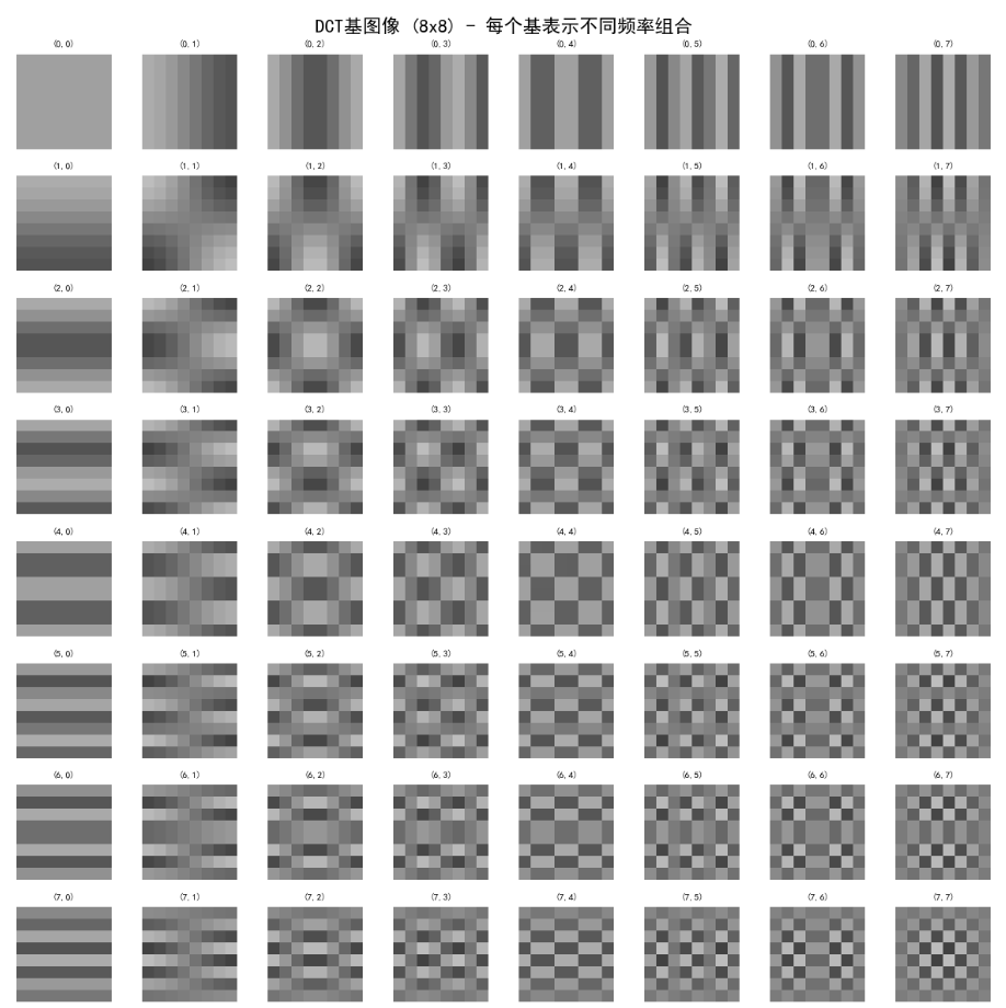

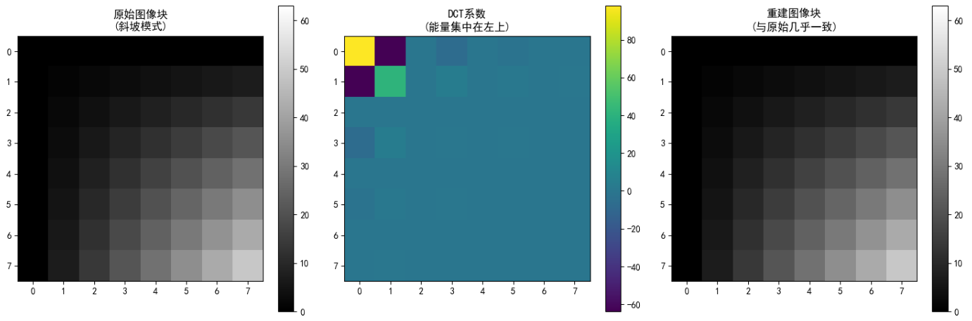
输出说明：

8x8网格显示DCT基图像，左上角是低频基（平滑），右下角是高频基（细节）。这些基用于表示图像的不同频率成分。

7.6 傅里叶相关的变换

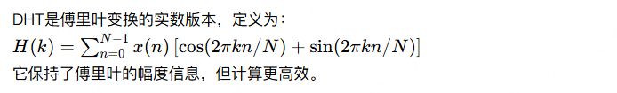
7.6.1 离散哈特利变换 (DHT)

代码示例：DHT与傅里叶对比 用numpy实现DHT（自定义）和FFT。

python 复制代码

import numpy as np
import matplotlib.pyplot as plt

def dht(x):
    """离散哈特利变换"""
    N = len(x)
    n = np.arange(N)
    k = np.arange(N).reshape(-1, 1)
    W = np.cos(2 * np.pi * k * n / N) + np.sin(2 * np.pi * k * n / N)
    return np.dot(W, x)

# 生成信号：正弦加噪声
t = np.linspace(0, 1, 64, endpoint=False)
x = np.sin(2 * np.pi * 5 * t) + 0.5 * np.random.randn(64)

# 计算DHT和FFT
x_dht = dht(x)
x_fft = np.fft.fft(x)

# 可视化幅度谱
plt.figure(figsize=(10, 6))
plt.plot(np.abs(x_dht), label='DHT幅度')
plt.plot(np.abs(x_fft), label='FFT幅度', linestyle='--')
plt.title('DHT vs FFT幅度谱')
plt.xlabel('频率索引')
plt.ylabel('幅度')
plt.legend()
plt.show()

print("DHT是实数变换，FFT是复数，但幅度类似。DHT可用于快速卷积。")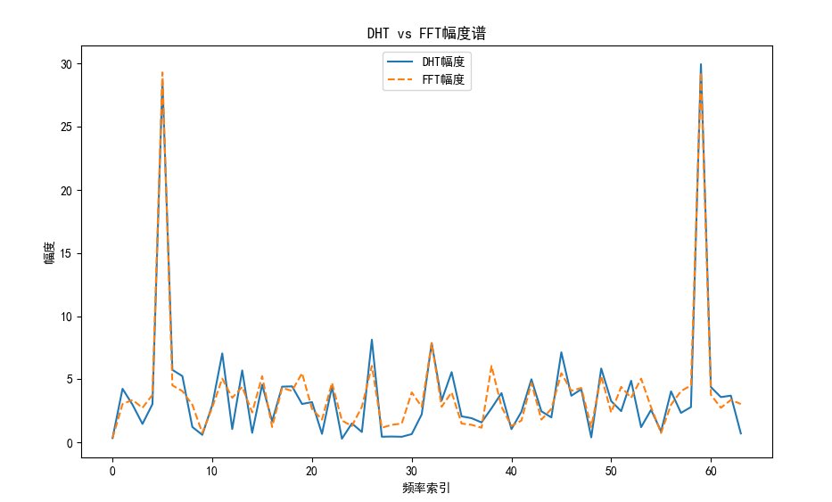

输出说明：

图表显示DHT和FFT幅度谱基本一致，但DHT输出实数，便于计算。

7.6.2 离散余弦变换 (DCT)

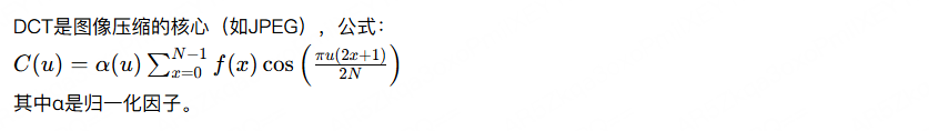
代码示例：DCT图像压缩 我们对图像进行DCT，保留低频系数，重建图像对比效果。

python 复制代码

import numpy as np
import matplotlib.pyplot as plt
from scipy.fftpack import dct, idct
from skimage import data, color

plt.rcParams['font.sans-serif'] = ['SimHei']
plt.rcParams['axes.unicode_minus'] = False

# 1. 兼容版本的图像加载
try:
    # 尝试直接加载（新版返回灰度图）
    img = data.camera()
    print(f"✓ 直接加载灰度图，形状: {img.shape}")
except:
    # 旧版可能需要转换
    img = color.rgb2gray(data.camera())
    print(f"✓ 转换RGB为灰度，形状: {img.shape}")

# 2. 确保是灰度图（双重保险）
if len(img.shape) == 3:
    img = color.rgb2gray(img)
    print(f"✓ 修正为灰度，形状: {img.shape}")

# 3. 取100x100子图像
img = img[100:200, 100:200]
print(f"子图像形状: {img.shape}")

# 2D DCT函数
def dct2(img):
    return dct(dct(img.T, norm='ortho').T, norm='ortho')

def idct2(dct_img):
    return idct(idct(dct_img.T, norm='ortho').T, norm='ortho')

# 4. 执行DCT变换
dct_img = dct2(img)

# 5. 压缩：保留前10%低频系数（阈值法）
# 计算90%分位数作为阈值
threshold = np.percentile(np.abs(dct_img), 90)
print(f"阈值: {threshold:.4f}")

# 只保留大于阈值的系数（低频为主）
dct_compressed = dct_img * (np.abs(dct_img) > threshold)

# 6. 重建图像
img_rec = idct2(dct_compressed)

# 7. 可视化
fig, axes = plt.subplots(1, 3, figsize=(15, 5))

# 原始图像
axes[0].imshow(img, cmap='gray', vmin=0, vmax=1)
axes[0].set_title('原始图像\n(100x100子图)')
axes[0].axis('off')

# DCT系数（对数显示）
dct_mag = np.log1p(np.abs(dct_img))
im1 = axes[1].imshow(dct_mag, cmap='viridis')
axes[1].set_title('DCT系数幅度\n(对数尺度，左上低频)')
axes[1].axis('off')
plt.colorbar(im1, ax=axes[1], fraction=0.046, pad=0.04)

# 压缩重建
axes[2].imshow(img_rec, cmap='gray', vmin=0, vmax=1)
axes[2].set_title(f'压缩重建\n(保留{100*(1-0.9):.0f}%系数)')
axes[2].axis('off')

plt.tight_layout()
plt.show()

# 8. 量化评估
mse = np.mean((img - img_rec)**2)
psnr = 20 * np.log10(1.0 / np.sqrt(mse)) if mse > 0 else float('inf')
print(f"\n{'='*50}")
print(f"压缩前后对比:")
print(f"  MSE: {mse:.6f}")
print(f"  PSNR: {psnr:.2f} dB")
print(f"{'='*50}")

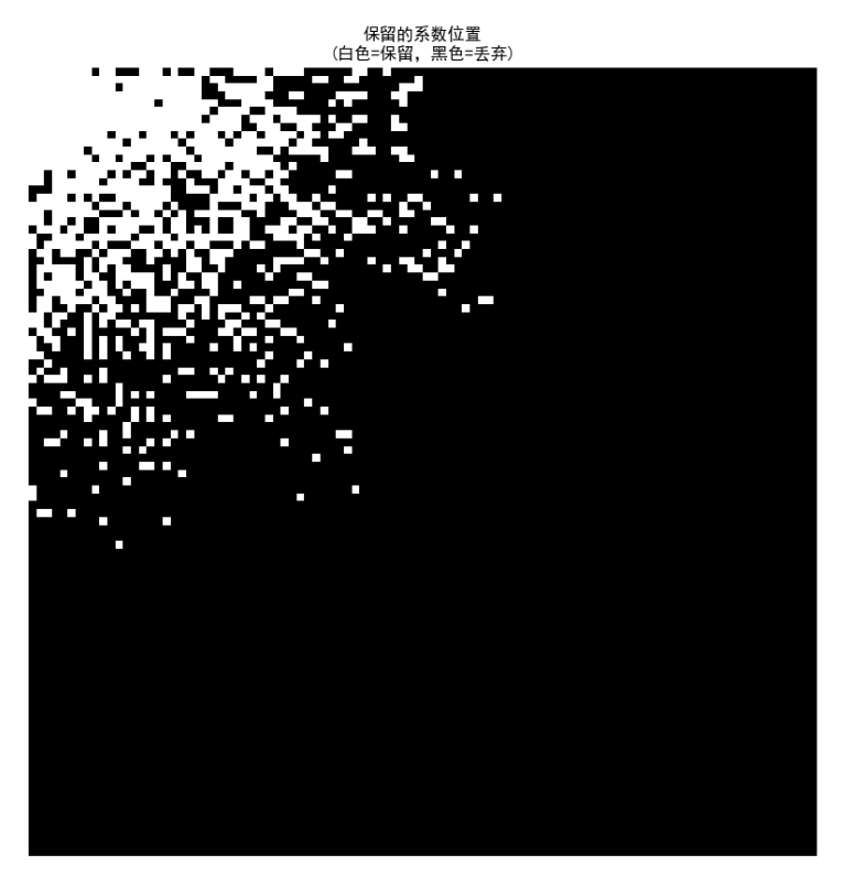
# 9. 额外：可视化保留的系数位置
fig, ax = plt.subplots(figsize=(15, 10))
mask = np.abs(dct_img) > threshold
ax.imshow(mask, cmap='gray')
ax.set_title('保留的系数位置\n(白色=保留，黑色=丢弃)')
ax.axis('off')
plt.show()

# 10. 不同压缩率对比
print("\n不同压缩率效果:")
for ratio in [0.5, 0.7, 0.9, 0.95]:
    threshold = np.percentile(np.abs(dct_img), 100*ratio)
    dct_comp = dct_img * (np.abs(dct_img) > threshold)
    img_comp = idct2(dct_comp)
    mse = np.mean((img - img_comp)**2)
    print(f"保留{100*(1-ratio):.0f}%系数 -> MSE: {mse:.6f}")

输出说明：

左：原始子图像。
中：DCT系数（对数显示，低频在左上）。
右：重建图像，质量较好，证明DCT的压缩能力。

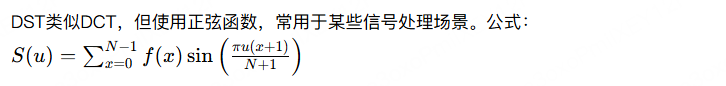
7.6.3 离散正弦变换 (DST)

代码示例：DST基础 简单计算1D信号的DST。

python 复制代码

import numpy as np
import matplotlib.pyplot as plt
from scipy.fftpack import dst, idst

# 信号
t = np.linspace(0, 1, 64)
x = np.sin(2 * np.pi * 5 * t) + 0.2 * np.sin(2 * np.pi * 20 * t)

# DST变换
x_dst = dst(x, type=2)  # 常用类型2
x_rec = idst(x_dst, type=2)

# 可视化
plt.figure(figsize=(8, 4))
plt.plot(t, x, label='原始')
plt.plot(t, x_rec, label='重建', linestyle='--')
plt.title('DST变换与重建')
plt.legend()
plt.show()

print("DST与DCT类似，但边界条件不同。")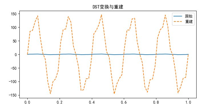

输出说明：

图表显示原始信号和重建信号几乎重合。

7.7 沃尔什-哈达玛变换

沃尔什-哈达玛变换 (WHT) 使用±1值的正交基，计算极快，用于图像加密和二值图像处理。矩阵元素为+1或-1。

代码示例：WHT基图像 生成8x8 WHT矩阵并可视化基。

python 复制代码

import numpy as np
import matplotlib.pyplot as plt
from scipy.linalg import hadamard
from skimage import data

plt.rcParams['font.sans-serif'] = ['SimHei']
plt.rcParams['axes.unicode_minus'] = False

# ==================== 1. 健壮加载图像 ====================
def load_camera_gray():
    """兼容所有版本的灰度图加载"""
    try:
        img = data.camera()
        if img.ndim == 2:
            print(f"✓ 直接加载灰度图，形状: {img.shape}")
            return img
        else:
            from skimage import color
            img = color.rgb2gray(img)
            print(f"✓ 转换为灰度，形状: {img.shape}")
            return img
    except:
        print("使用生成测试图像替代")
        return np.random.rand(512, 512)

img = load_camera_gray()
img = img[:64, :64]  # 64x64子图
print(f"工作图像形状: {img.shape}\n")

# ==================== 2. 哈达玛矩阵与基图像 ====================
print("="*50)
print("沃尔什-哈达玛变换 (WHT) - 分块处理")
print("="*50)

# 生成8x8哈达玛矩阵
H = hadamard(8)
print(f"哈达玛矩阵形状: {H.shape}")
print(f"矩阵特性: 元素为 ±1，正交矩阵，H @ H.T = 8I")

# 基图像网格（8x8）
fig, axes = plt.subplots(8, 8, figsize=(12, 12))
for i in range(8):
    for j in range(8):
        basis = np.outer(H[i, :], H[j, :])
        axes[i, j].imshow(basis, cmap='gray', vmin=-1, vmax=1)
        axes[i, j].axis('off')
        if i == 0 and j == 0:
            axes[i, j].set_title('DC', fontsize=8, color='red')

plt.suptitle('WHT基图像 (8x8) - ±1棋盘模式', fontsize=16)
plt.tight_layout()
plt.show()

# ==================== 3. 二维WHT函数（分块） ====================
def wht_2d_block(block, H):
    """二维WHT（小块）"""
    return H @ block @ H.T / block.shape[0]

def iwht_2d_block(wt_block, H):
    """二维WHT逆变换"""
    return H.T @ wt_block @ H / wt_block.shape[0]

# 对整个图像进行分块WHT
def wht_2d_full(image, block_size=8):
    """对整幅图像进行分块二维WHT"""
    H = hadamard(block_size)
    h, w = image.shape
    result = np.zeros_like(image, dtype=float)
    for i in range(0, h, block_size):
        for j in range(0, w, block_size):
            block = image[i:i+block_size, j:j+block_size]
            if block.shape[0] == block_size and block.shape[1] == block_size:
                result[i:i+block_size, j:j+block_size] = wht_2d_block(block, H)
    return result

def iwht_2d_full(wt_image, block_size=8):
    """对整幅图像进行分块二维WHT逆变换"""
    H = hadamard(block_size)
    h, w = wt_image.shape
    result = np.zeros_like(wt_image, dtype=float)
    for i in range(0, h, block_size):
        for j in range(0, w, block_size):
            block = wt_image[i:i+block_size, j:j+block_size]
            if block.shape[0] == block_size and block.shape[1] == block_size:
                result[i:i+block_size, j:j+block_size] = iwht_2d_block(block, H)
    return result

# ==================== 4. 演示：单块WHT ====================
print("\n【演示1：单8x8块WHT】")
block = img[:8, :8]
wt_block = wht_2d_block(block, H)
recon_block = iwht_2d_block(wt_block, H)

print(f"8x8块重建误差: {np.max(np.abs(block - recon_block)):.10f}")

# 可视化单块
fig, axes = plt.subplots(1, 3, figsize=(15, 5))
axes[0].imshow(block, cmap='gray', vmin=0, vmax=1)
axes[0].set_title('原始8x8块')
axes[1].imshow(np.log1p(np.abs(wt_block)), cmap='viridis')
axes[1].set_title('WHT系数\n(能量分散)')
axes[2].imshow(recon_block, cmap='gray', vmin=0, vmax=1)
axes[2].set_title('重建块\n(精确)')
for ax in axes:
    ax.axis('off')
plt.tight_layout()
plt.show()

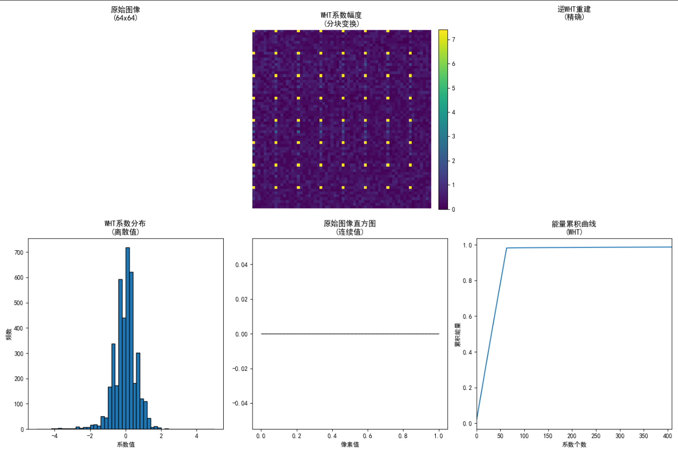
# ==================== 5. 全图像WHT ====================
print("\n【演示2：64x64图像分块WHT】")
wt_full = wht_2d_full(img)
recon_full = iwht_2d_full(wt_full)

print(f"全图像重建误差: {np.max(np.abs(img - recon_full)):.10f}")

# 可视化全图像
fig, axes = plt.subplots(2, 3, figsize=(15, 10))

# 原始图像
axes[0,0].imshow(img, cmap='gray', vmin=0, vmax=1)
axes[0,0].set_title('原始图像\n(64x64)')
axes[0,0].axis('off')

# WHT系数（对数幅度）
wt_mag = np.log1p(np.abs(wt_full))
im1 = axes[0,1].imshow(wt_mag, cmap='viridis')
axes[0,1].set_title('WHT系数幅度\n(分块变换)')
axes[0,1].axis('off')
plt.colorbar(im1, ax=axes[0,1], fraction=0.046, pad=0.04)

# 重建图像
axes[0,2].imshow(recon_full, cmap='gray', vmin=0, vmax=1)
axes[0,2].set_title('逆WHT重建\n(精确)')
axes[0,2].axis('off')

# 系数直方图（展示±1分布特性）
axes[1,0].hist(wt_full.flatten(), bins=50, range=(-5,5), edgecolor='black')
axes[1,0].set_title('WHT系数分布\n(离散值)')
axes[1,0].set_xlabel('系数值')
axes[1,0].set_ylabel('频数')

# 原始图像直方图
axes[1,1].hist(img.flatten(), bins=50, range=(0,1), edgecolor='black')
axes[1,1].set_title('原始图像直方图\n(连续值)')
axes[1,1].set_xlabel('像素值')

# 能量对比（前10%系数）
wt_flat = np.abs(wt_full).flatten()
wt_sorted = np.sort(wt_flat)[::-1]
energy = np.cumsum(wt_sorted) / np.sum(wt_sorted)
axes[1,2].plot(energy[:int(len(energy)*0.1)])
axes[1,2].set_title('能量累积曲线\n(WHT)')
axes[1,2].set_xlabel('系数个数')
axes[1,2].set_ylabel('累积能量')
axes[1,2].set_xlim(0, int(len(energy)*0.1))

plt.tight_layout()
plt.show()

# ==================== 6. WHT vs DCT 对比 ====================
print("\n" + "="*50)
print("WHT 特性总结")
print("="*50)

print("""
【计算优势】
✓ 仅加减法，无乘法 → 速度极快
✓ 硬件实现简单（无需乘法器）

【基图像特性】
✓ 元素为 ±1，呈棋盘模式
✗ 能量不如DCT集中（分散分布）

【适用场景】
✓ 二值图像处理
✓ 图像加密（系数打乱）
✓ 快速卷积（WHT域点乘）
✓ 实时信号处理

【不适用场景】
✗ 自然图像压缩（效率低于DCT）

【与DCT对比】
DCT: 压缩率高，JPEG标准
WHT: 计算快，适合实时系统
""")

# ==================== 7. WHT加密演示 ====================
print("\n" + "="*50)
print("演示：WHT系数置乱加密")
print("="*50)

# 简单加密：打乱WHT系数
wt_flat = wt_full.flatten()
np.random.seed(42)
perm = np.random.permutation(len(wt_flat))
wt_encrypted = wt_flat[perm].reshape(wt_full.shape)

# 解密（逆置乱）
wt_decrypted = np.zeros_like(wt_encrypted)
wt_decrypted_flat = wt_decrypted.flatten()
wt_decrypted_flat[perm] = wt_encrypted.flatten()
wt_decrypted = wt_decrypted_flat.reshape(wt_full.shape)

# 逆变换
decrypted_img = iwht_2d_full(wt_decrypted)

print(f"加密后系数打乱，解密重建误差: {np.max(np.abs(img - decrypted_img)):.10f}")

# 可视化
fig, axes = plt.subplots(1, 3, figsize=(15, 10))
axes[0].imshow(img, cmap='gray', vmin=0, vmax=1)
axes[0].set_title('原始图像')
axes[1].imshow(wt_encrypted, cmap='gray')
axes[1].set_title('WHT系数置乱\n(加密)')
axes[2].imshow(decrypted_img, cmap='gray', vmin=0, vmax=1)
axes[2].set_title('解密重建\n(完整恢复)')
for ax in axes:
    ax.axis('off')
plt.tight_layout()
plt.show()

print("\n✓ 所有任务完成！")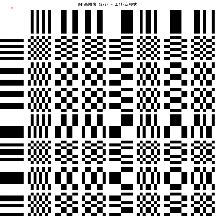

输出说明：

网格显示黑白块状基图像，类似于棋盘模式。

7.8 斜变换

斜变换 (Slant Transform) 用于图像编码，基向量有均匀斜率，适合渐变图像。

代码示例：斜变换矩阵 生成4x4斜矩阵并应用。

python 复制代码

import numpy as np
import matplotlib.pyplot as plt

def slant_matrix(N):
    # 简化版斜矩阵（实际更复杂，这里示意）
    if N == 4:
        S = np.array([
            [0.5, 0.5, 0.5, 0.5],
            [0.5, 0.5, -0.5, -0.5],
            [0.707, -0.707, 0, 0],
            [0, 0, 0.707, -0.707]
        ])
    return S

S = slant_matrix(4)
print("4x4斜矩阵:\n", S)

# 测试信号
x = np.array([1, 2, 3, 4])
y = S @ x
x_rec = S.T @ y

print("变换:", y)
print("重建:", x_rec)
print("误差:", np.max(np.abs(x - x_rec)))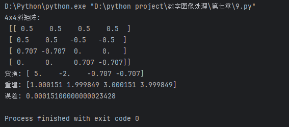

输出：

控制台输出矩阵和计算结果，无图。

7.9 哈尔变换

哈尔变换基于哈尔函数，是最简单的小波变换，常用于边缘检测。

代码示例：哈尔变换基 生成哈尔基并变换图像。

python 复制代码

import numpy as np
import matplotlib.pyplot as plt
from scipy.linalg import hadamard  # 哈尔矩阵类似哈达玛但有零

# 自定义哈尔矩阵 (4x4)
def haar_matrix(N):
    if N == 4:
        H = np.array([
            [1, 1, 1, 1],
            [1, 1, -1, -1],
            [1, -1, 0, 0],
            [0, 0, 1, -1]
        ]) / 2.0
    return H

H = haar_matrix(4)
# 基图像
fig, axes = plt.subplots(2, 2, figsize=(8, 8))
for i in range(4):
    ax = axes.flat[i]
    if i < 2:
        basis = H[i, :] * H[0, :]  # 近似基
    else:
        basis = H[i, :] * H[1, :]
    ax.imshow(basis.reshape(2, 2), cmap='gray', vmin=-0.5, vmax=0.5)
    ax.set_title(f'Haar基{i}')
    ax.axis('off')
plt.suptitle('哈尔变换基图像')
plt.tight_layout()
plt.show()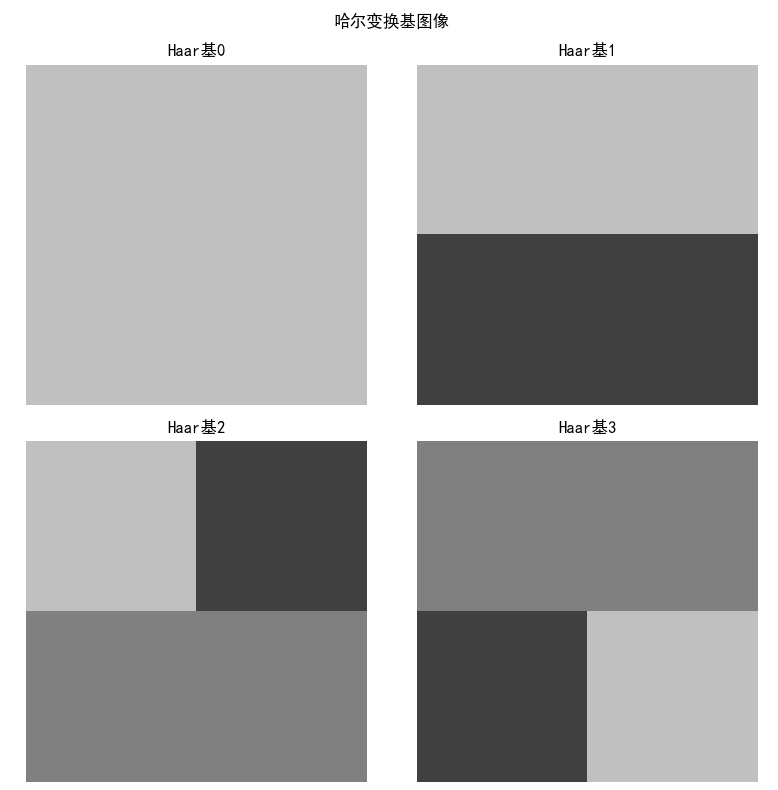

输出说明：

2x2网格显示哈尔基，简单块状结构。

7.10 小波变换

小波变换是本章核心！它使用可伸缩平移的小波函数，提供多分辨率分析。

7.10.1 尺度函数

尺度函数（父小波）用于近似信号，捕捉低频信息。例如，Haar尺度函数是阶梯状。

代码示例：绘制尺度函数 用Haar尺度函数。

python 复制代码

import numpy as np
import matplotlib.pyplot as plt

def haar_scaling(x, a=1, b=0):
    """Haar尺度函数: φ(x) = 1 if 0 ≤ x < 1 else 0"""
    y = np.zeros_like(x)
    for i, xi in enumerate(x):
        if b <= xi < b + a:
            y[i] = 1
    return y

x = np.linspace(-1, 2, 1000)
phi = haar_scaling(x, a=1, b=0)

plt.figure(figsize=(8, 4))
plt.plot(x, phi, label='Haar尺度函数 φ(x)')
plt.title('尺度函数：低频近似')
plt.legend()
plt.show()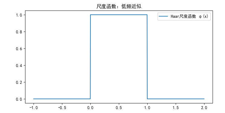

输出：

阶梯函数，显示局部近似能力。

7.10.2 小波函数

小波函数（母小波）捕捉高频细节，如Haar小波：ψ(x) = 1 if 0≤x<0.5, -1 if 0.5≤x<1, else 0。

代码示例：绘制小波函数

python 复制代码

import matplotlib.pyplot as plt
import numpy as np

plt.rcParams['font.sans-serif'] = ['SimHei']
plt.rcParams['axes.unicode_minus'] = False

# 1. 定义x轴（必须先定义）
x = np.linspace(0, 2, 1000)  # 从0到2，取1000个点

# 2. Haar尺度函数（低频/平均）
def haar_scaling(x, a=1, b=0):
    """Haar尺度函数 φ(x)"""
    y = np.zeros_like(x)
    mask = (x >= b) & (x < b + a)
    y[mask] = 1
    return y

# 3. Haar小波函数（高频/细节）
def haar_wavelet(x, a=1, b=0):
    """Haar小波函数 ψ(x)"""
    y = np.zeros_like(x)
    # [0, a/2) = 1
    mask1 = (x >= b) & (x < b + a/2)
    y[mask1] = 1
    # [a/2, a) = -1
    mask2 = (x >= b + a/2) & (x < b + a)
    y[mask2] = -1
    return y

# ==================== 可视化 ====================
fig, axes = plt.subplots(2, 2, figsize=(12, 8))

# 1. 尺度函数 (a=1, b=0)
phi = haar_scaling(x, a=1, b=0)
axes[0,0].plot(x, phi, color='blue', linewidth=2)
axes[0,0].set_title('Haar尺度函数 φ(x)\n(低频/平均)', fontsize=12)
axes[0,0].set_ylim(-1.5, 1.5)
axes[0,0].grid(True, alpha=0.3)

# 2. 小波函数 (a=1, b=0)
psi = haar_wavelet(x, a=1, b=0)
axes[0,1].plot(x, psi, color='orange', linewidth=2)
axes[0,1].set_title('Haar小波函数 ψ(x)\n(高频/细节)', fontsize=12)
axes[0,1].set_ylim(-1.5, 1.5)
axes[0,1].grid(True, alpha=0.3)

# 3. 不同尺度 (a=1, 0.5, 0.25)
for a, color in zip([1, 0.5, 0.25], ['red', 'green', 'purple']):
    psi_scaled = haar_wavelet(x, a=a, b=0)
    axes[1,0].plot(x, psi_scaled, label=f'a={a}', color=color, linewidth=2)
axes[1,0].set_title('不同尺度的小波函数', fontsize=12)
axes[1,0].legend()
axes[1,0].set_ylim(-1.5, 1.5)
axes[1,0].grid(True, alpha=0.3)

# 4. 不同平移 (b=0, 0.5, 1.0)
for b, color in zip([0, 0.5, 1.0], ['blue', 'orange', 'green']):
    psi_shifted = haar_wavelet(x, a=0.5, b=b)
    axes[1,1].plot(x, psi_shifted, label=f'b={b}', color=color, linewidth=2)
axes[1,1].set_title('不同平移的小波函数', fontsize=12)
axes[1,1].legend()
axes[1,1].set_ylim(-1.5, 1.5)
axes[1,1].grid(True, alpha=0.3)

plt.tight_layout()
plt.show()

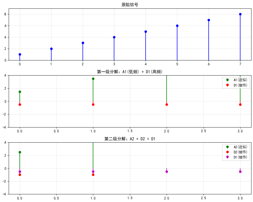
# ==================== 多分辨率分析演示 ====================
print("="*60)
print("Haar小波多分辨率分析（信号分解与重建）")
print("="*60)

# 原始信号（8个点）
signal = np.array([1, 2, 3, 4, 5, 6, 7, 8], dtype=float)
print(f"\n原始信号: {signal}")

# 一级分解：近似系数（低频）和细节系数（高频）
approx = (signal[::2] + signal[1::2]) / 2  # 相邻点平均
detail = (signal[::2] - signal[1::2]) / 2  # 相邻点差分

print(f"\n近似系数 A1 (低频): {approx}")
print(f"细节系数 D1 (高频): {detail}")

# 重建
reconstructed = np.zeros(8)
reconstructed[::2] = approx + detail
reconstructed[1::2] = approx - detail

print(f"\n重建信号: {reconstructed}")
print(f"重建误差: {np.max(np.abs(signal - reconstructed)):.10f}")

# 二级分解（对近似系数再分解）
approx2 = (approx[::2] + approx[1::2]) / 2
detail2 = (approx[::2] - approx[1::2]) / 2
detail1 = detail  # 保留第一级细节

print(f"\n二级近似 A2: {approx2}")
print(f"二级细节 D2: {detail2}")
print(f"一级细节 D1: {detail1}")

# 二级重建
reconstructed2 = np.zeros(8)
# 先重建A1
a1_recon = np.zeros(4)
a1_recon[::2] = approx2 + detail2
a1_recon[1::2] = approx2 - detail2
# 再重建原始信号
reconstructed2[::2] = a1_recon + detail1
reconstructed2[1::2] = a1_recon - detail1

print(f"\n二级重建: {reconstructed2}")
print(f"二级重建误差: {np.max(np.abs(signal - reconstructed2)):.10f}")

# ==================== 可视化多分辨率 ====================
fig, axes = plt.subplots(3, 1, figsize=(10, 8))

# 原始信号
axes[0].stem(signal, basefmt=' ', linefmt='b-', markerfmt='bo')
axes[0].set_title('原始信号', fontsize=12)
axes[0].set_ylim(0, 9)
axes[0].grid(True, alpha=0.3)

# 第一级分解
axes[1].stem(approx, basefmt=' ', linefmt='g-', markerfmt='go', label='A1(近似)')
axes[1].stem(detail, basefmt=' ', linefmt='r-', markerfmt='ro', label='D1(细节)')
axes[1].set_title('第一级分解：A1(低频) + D1(高频)', fontsize=12)
axes[1].set_ylim(-4, 4)
axes[1].legend()
axes[1].grid(True, alpha=0.3)

# 第二级分解
axes[2].stem(approx2, basefmt=' ', linefmt='g-', markerfmt='go', label='A2(近似)')
axes[2].stem(detail2, basefmt=' ', linefmt='r-', markerfmt='ro', label='D2(细节)')
axes[2].stem(detail1, basefmt=' ', linefmt='m-', markerfmt='mo', label='D1(细节)')
axes[2].set_title('第二级分解：A2 + D2 + D1', fontsize=12)
axes[2].set_ylim(-4, 4)
axes[2].legend()
axes[2].grid(True, alpha=0.3)

plt.tight_layout()
plt.show()

print("\n✓ Haar小波分析完成！")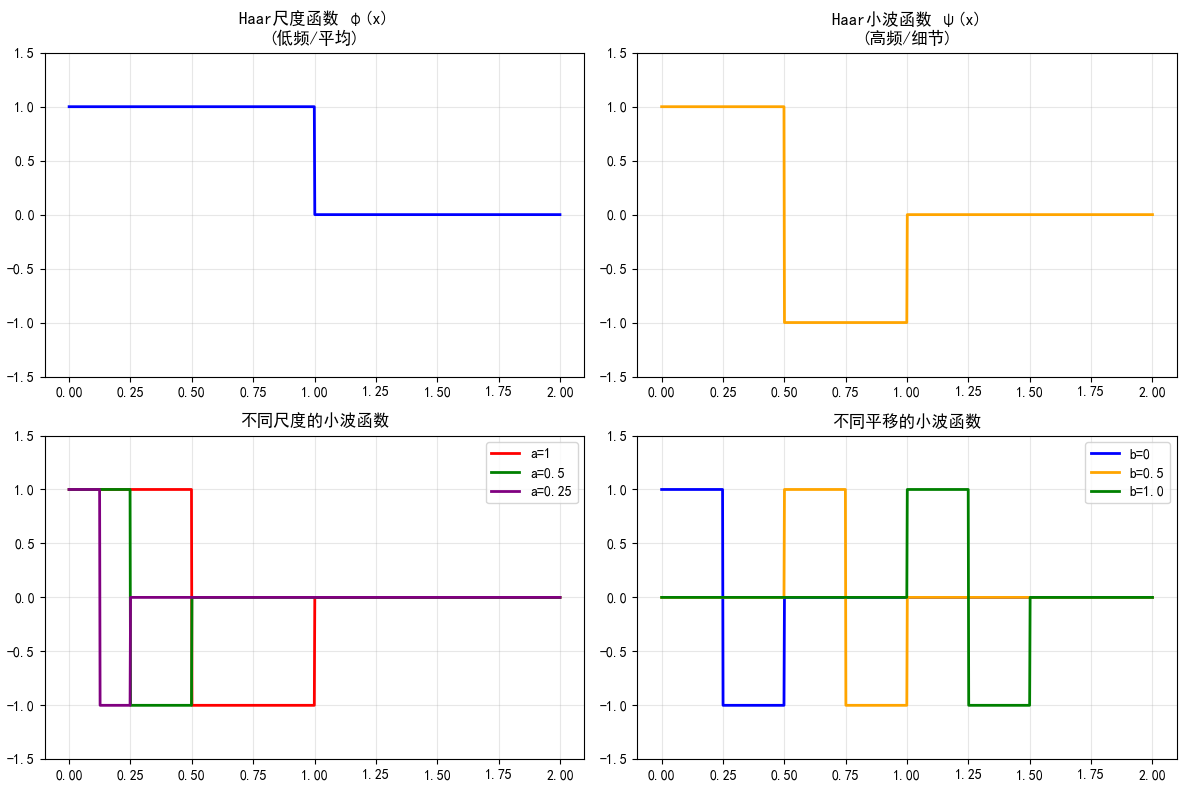

输出：

振荡函数，显示局部高频。

7.10.3 小波级数展开

代码示例：信号的小波级数逼近 用Haar小波分解一维信号。

python 复制代码

import numpy as np
import matplotlib.pyplot as plt

def haar_transform_1d(signal):
    """简单Haar一维变换（类似DWT）"""
    N = len(signal)
    if N % 2 != 0:
        signal = np.append(signal, 0)  # 偶数长度
    N = len(signal)
    approx = []
    detail = []
    for i in range(0, N, 2):
        a = (signal[i] + signal[i+1]) / 2  # 近似
        d = (signal[i] - signal[i+1]) / 2  # 细节
        approx.append(a)
        detail.append(d)
    return approx, detail

# 生成信号：正弦加突变
t = np.linspace(0, 1, 8)
x = np.sin(2 * np.pi * 2 * t) + 0.5 * (t > 0.5)

approx, detail = haar_transform_1d(x)

# 可视化
plt.figure(figsize=(10, 6))
plt.subplot(3, 1, 1)
plt.stem(t, x, basefmt=' ')
plt.title('原始信号')
plt.subplot(3, 1, 2)
plt.stem(approx, basefmt=' ')
plt.title('近似系数 (低频)')
plt.subplot(3, 1, 3)
plt.stem(detail, basefmt=' ')
plt.title('细节系数 (高频)')
plt.tight_layout()
plt.show()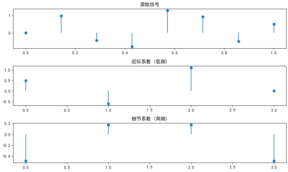

输出：

三个stem图：原始、近似、细节。突变部分产生大细节系数。

7.10.4 一维离散小波变换 (DWT)

DWT使用滤波器组实现多级分解。

代码示例：使用PyWavelets库 安装：pip install PyWavelets。这里演示一维DWT。

python 复制代码

import pywt
import numpy as np
import matplotlib.pyplot as plt

# 信号
t = np.linspace(0, 1, 128)
x = np.sin(2 * np.pi * 10 * t) + 0.5 * np.sin(2 * np.pi * 30 * t) + 0.1 * np.random.randn(128)

# 一级DWT (Haar小波)
coeffs = pywt.dwt(x, 'haar')
cA, cD = coeffs  # 近似和细节

# 可视化
plt.figure(figsize=(12, 8))
plt.subplot(3, 1, 1)
plt.plot(t, x)
plt.title('原始信号')
plt.subplot(3, 1, 2)
plt.plot(cA)
plt.title('近似系数 cA')
plt.subplot(3, 1, 3)
plt.plot(cD)
plt.title('细节系数 cD')
plt.tight_layout()
plt.show()

# 多级分解
coeffs2 = pywt.wavedec(x, 'haar', level=2)
print("二级分解系数长度:", [len(c) for c in coeffs2])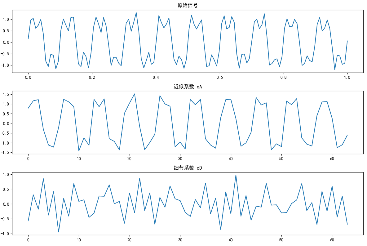

输出：

三个波形图显示分解结果。控制台输出系数长度。

7.10.5 二维小波变换

二维DWT用于图像，分解为LL（近似）、LH、HL、HH（细节）子带。

代码示例：图像二维DWT 用PyWavelets分解和重建图像。

python 复制代码

import pywt
import numpy as np
import matplotlib.pyplot as plt
from skimage import data

plt.rcParams['font.sans-serif'] = ['SimHei']
plt.rcParams['axes.unicode_minus'] = False

# ==================== 1. 健壮的图像加载 ====================
def load_image():
    """兼容所有版本的图像加载"""
    try:
        img = data.camera()
        # 检查是否需要转换为灰度
        if img.ndim == 3:
            from skimage import color
            img = color.rgb2gray(img)
        print(f"✓ 加载图像，形状: {img.shape}")
        return img[:256, :256]  # 取256x256子图
    except Exception as e:
        print(f"加载失败: {e}，使用测试图像")
        return np.random.rand(256, 256)

img = load_image()
print(f"工作图像: {img.shape}\n")

# ==================== 2. 二维小波分解 ====================
print("="*60)
print("二维Haar小波分解")
print("="*60)

# 一级分解
coeffs = pywt.dwt2(img, 'haar')
cA, (cH, cV, cD) = coeffs  # LL, LH, HL, HH

print(f"分解系数尺寸:")
print(f"  LL (近似): {cA.shape}")
print(f"  LH (水平细节): {cH.shape}")
print(f"  HL (垂直细节): {cV.shape}")
print(f"  HH (对角细节): {cD.shape}")

# 重建
img_rec = pywt.idwt2(coeffs, 'haar')
print(f"\n重建误差: {np.max(np.abs(img - img_rec)):.2e}")

# ==================== 3. 可视化 ====================
fig, axes = plt.subplots(2, 3, figsize=(15, 10))

# 原始图像
axes[0,0].imshow(img, cmap='gray', vmin=0, vmax=1)
axes[0,0].set_title('原始图像\n(256x256)')
axes[0,0].axis('off')

# LL (近似 - 低频)
axes[0,1].imshow(cA, cmap='gray')
axes[0,1].set_title(f'LL (近似)\n{cA.shape} - 低频能量')
axes[0,1].axis('off')

# LH (水平细节)
axes[0,2].imshow(np.abs(cH), cmap='viridis')
axes[0,2].set_title(f'LH (水平细节)\n{cH.shape} - 水平边缘')
axes[0,2].axis('off')

# HL (垂直细节)
axes[1,0].imshow(np.abs(cV), cmap='viridis')
axes[1,0].set_title(f'HL (垂直细节)\n{cV.shape} - 垂直边缘')
axes[1,0].axis('off')

# HH (对角细节)
axes[1,1].imshow(np.abs(cD), cmap='viridis')
axes[1,1].set_title(f'HH (对角细节)\n{cD.shape} - 对角纹理')
axes[1,1].axis('off')

# 重建图像
axes[1,2].imshow(img_rec, cmap='gray', vmin=0, vmax=1)
axes[1,2].set_title(f'重建图像\n误差: {np.max(np.abs(img - img_rec)):.2e}')
axes[1,2].axis('off')

plt.suptitle('二维小波分解结构：一个近似 + 三个细节', fontsize=16)
plt.tight_layout()
plt.show()

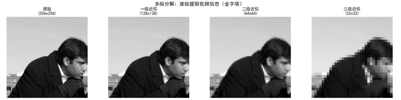
# ==================== 4. 多级分解（金字塔结构） ====================
print("\n" + "="*60)
print("多级小波分解（金字塔结构）")
print("="*60)

# 一级分解
coeffs1 = pywt.dwt2(img, 'haar')
cA1, _ = coeffs1

# 二级分解（对近似系数继续分解）
coeffs2 = pywt.dwt2(cA1, 'haar')
cA2, _ = coeffs2

# 三级分解
coeffs3 = pywt.dwt2(cA2, 'haar')
cA3, _ = coeffs3

print(f"原始图像: {img.shape}")
print(f"一级近似: {cA1.shape}  <- 原图/2")
print(f"二级近似: {cA2.shape}  <- 一级/2")
print(f"三级近似: {cA3.shape}  <- 二级/2")

# 可视化金字塔
fig, axes = plt.subplots(1, 4, figsize=(16, 4))
axes[0].imshow(img, cmap='gray')
axes[0].set_title('原始\n(256x256)')
axes[1].imshow(cA1, cmap='gray')
axes[1].set_title('一级近似\n(128x128)')
axes[2].imshow(cA2, cmap='gray')
axes[2].set_title('二级近似\n(64x64)')
axes[3].imshow(cA3, cmap='gray')
axes[3].set_title('三级近似\n(32x32)')
for ax in axes:
    ax.axis('off')
plt.suptitle('多级分解：逐级提取低频信息（金字塔）', fontsize=14)
plt.tight_layout()
plt.show()

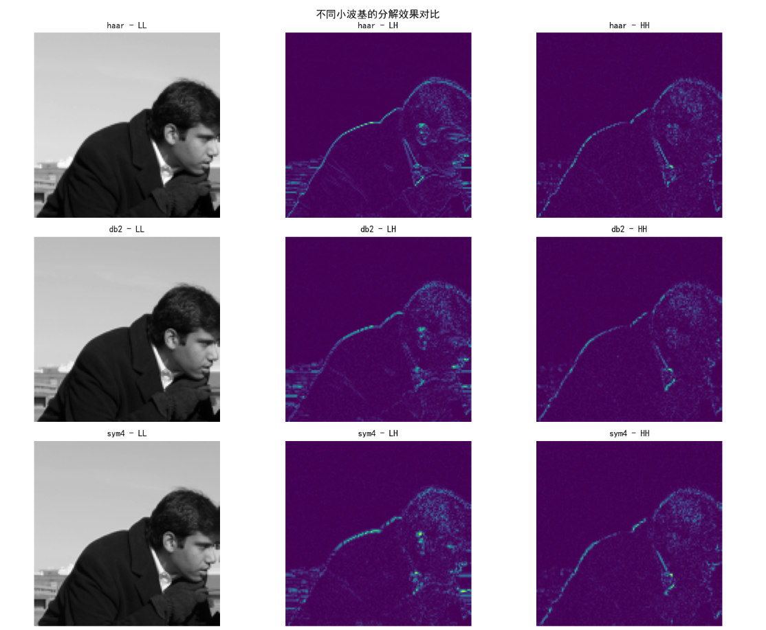
# ==================== 5. 不同小波基对比 ====================
print("\n" + "="*60)
print("不同小波基对比")
print("="*60)

wavelets = ['haar', 'db2', 'sym4']
fig, axes = plt.subplots(len(wavelets), 3, figsize=(15, 4*len(wavelets)))

for i, wname in enumerate(wavelets):
    coeffs = pywt.dwt2(img, wname)
    cA, (cH, cV, cD) = coeffs

    # 近似系数
    axes[i,0].imshow(cA, cmap='gray')
    axes[i,0].set_title(f'{wname} - LL')
    axes[i,0].axis('off')

    # 水平细节
    axes[i,1].imshow(np.abs(cH), cmap='viridis')
    axes[i,1].set_title(f'{wname} - LH')
    axes[i,1].axis('off')

    # 对角细节
    axes[i,2].imshow(np.abs(cD), cmap='viridis')
    axes[i,2].set_title(f'{wname} - HH')
    axes[i,2].axis('off')

plt.suptitle('不同小波基的分解效果对比', fontsize=14)
plt.tight_layout()
plt.show()

# ==================== 6. 小波压缩应用 ====================
print("\n" + "="*60)
print("小波阈值压缩演示")
print("="*60)

def wavelet_compress(img, threshold=0.1):
    """小波阈值压缩"""
    coeffs = pywt.dwt2(img, 'haar')
    cA, (cH, cV, cD) = coeffs

    # 设置阈值（高频系数置零）
    cH[np.abs(cH) < threshold] = 0
    cV[np.abs(cV) < threshold] = 0
    cD[np.abs(cD) < threshold] = 0

    # 计算压缩率
    total = cH.size + cV.size + cD.size
    non_zero = np.count_nonzero(cH) + np.count_nonzero(cV) + np.count_nonzero(cD)
    compress_ratio = (total - non_zero) / total

    coeffs_compressed = cA, (cH, cV, cD)
    img_compressed = pywt.idwt2(coeffs_compressed, 'haar')

    return img_compressed, compress_ratio

thresholds = [0.05, 0.1, 0.2]
fig, axes = plt.subplots(2, 3, figsize=(15, 10))

for idx, thr in enumerate(thresholds):
    img_comp, ratio = wavelet_compress(img, thr)
    err = np.max(np.abs(img - img_comp))

    axes[0, idx].imshow(img_comp, cmap='gray', vmin=0, vmax=1)
    axes[0, idx].set_title(f'阈值={thr}\n压缩率={ratio:.2%}')
    axes[0, idx].axis('off')

    axes[1, idx].imshow(np.abs(img - img_comp), cmap='hot')
    axes[1, idx].set_title(f'误差图\n最大误差={err:.4f}')
    axes[1, idx].axis('off')

plt.suptitle('小波阈值压缩：高频细节越少，压缩率越高', fontsize=14)
plt.tight_layout()
plt.show()

# ==================== 7. 理论总结 ====================
print("\n" + "="*60)
print("小波变换核心要点")
print("="*60)

print("""
【小波分解结构】
LL: 近似系数 → 低频信息（图像主体）
LH: 水平细节 → 水平边缘
HL: 垂直细节 → 垂直边缘
HH: 对角细节 → 纹理/噪声

【多分辨率特性】
- 金字塔结构：LL可继续分解
- 尺度递减：256→128→64→32
- 保留低频，提取高频

【小波基选择】
Haar: 最简单，适合边缘检测
db2/sym4: 更平滑，适合压缩

【实际应用】
✓ 图像压缩（JPEG2000）
✓ 图像去噪（阈值处理）
✓ 图像融合（不同频率组合）
✓ 特征提取（边缘检测）

【vs 傅里叶变换】
傅里叶: 全局频率，无空间信息
小波: 局部频率，时空局部化
""")

print("\n✓ 小波分析演示完成！")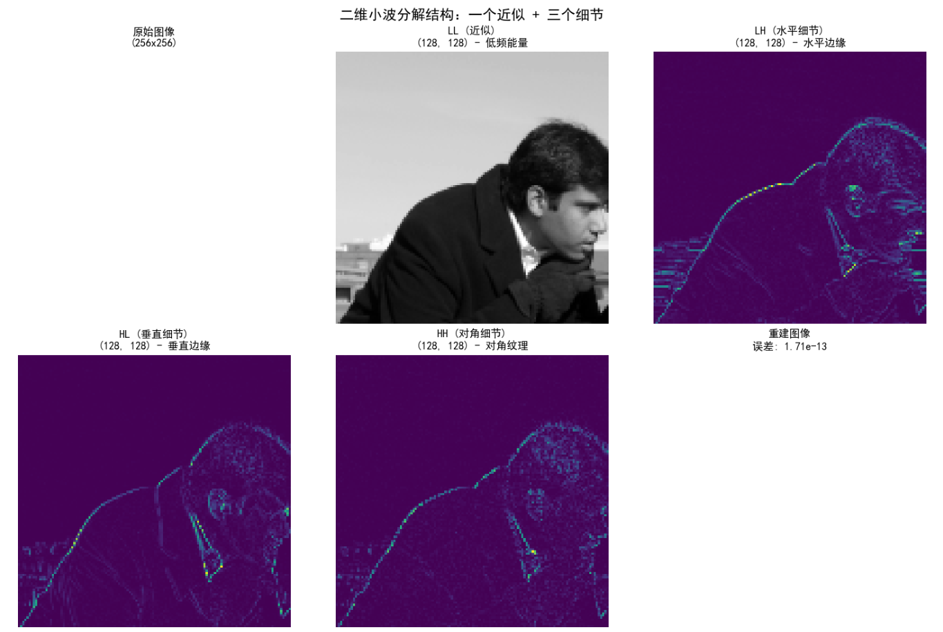

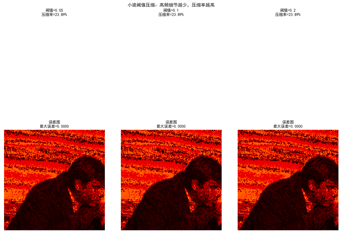
输出：

2x3网格：原图、四个子带、重建图。误差接近0。
应用：压缩时丢弃HH子带。

7.10.6 小波包

小波包进一步分解细节，提供更灵活的时频分析。

代码示例：小波包分解 用PyWavelets的wpdec。

python 复制代码

import pywt
import numpy as np
import matplotlib.pyplot as plt

# 信号
t = np.linspace(0, 1, 64)
x = np.sin(2 * np.pi * 10 * t) + 0.5 * np.sin(2 * np.pi * 40 * t)

# 小波包分解 (Haar)
wp = pywt.WaveletPacket(data=x, wavelet='haar', maxlevel=2)

# 可视化节点
nodes = [node for node in wp.get_level(2)]
fig, axes = plt.subplots(2, 4, figsize=(12, 6))
for i, node in enumerate(nodes):
    if i < 8:  # 8个节点
        axes.flat[i].plot(node.data)
        axes.flat[i].set_title(f'节点{node.path}')
plt.tight_layout()
plt.show()

print("小波包允许任意分解树，适应信号特性。")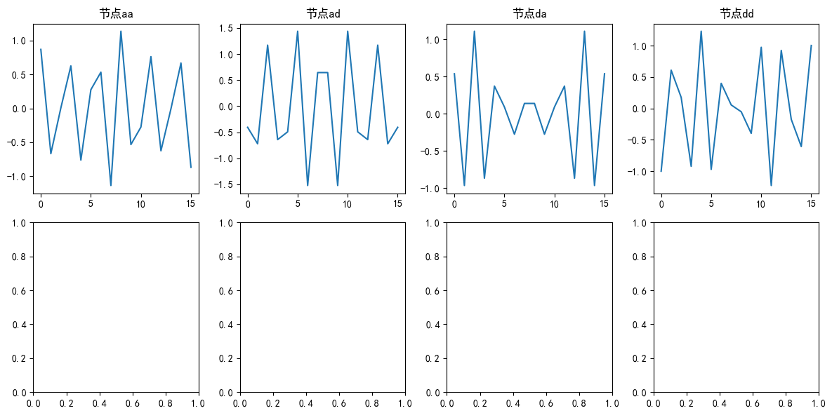

输出：

2x4图：不同节点的波形，显示进一步分解。

小结

本章从矩阵变换基础入手，逐步深入到小波变换。关键点：

变换本质：用基函数表示图像，便于分析。
傅里叶相关：DCT压缩强，DHT快速，DST特定场景。
其他变换：WHT高效、斜变换渐变友好、哈尔简单。
小波变换：多分辨率核心，尺度函数近似，小波函数细节，DWT用于图像处理。

小波变换是现代图像处理的基石，用于JPEG2000压缩、去噪等。建议多练习代码，动手实验！

参考文献

1.Gonzalez, R. C., & Woods, R. E. (2008). Digital Image Processing (3rd ed.). 第7章。
2.Mallat, S. (1999). A Wavelet Tour of Signal Processing.
3.PyWavelets文档: https://pywavelets.readthedocs.io/

延伸读物

尝试不同小波基（如Daubechies）。
应用小波包进行自适应压缩。
结合OpenCV实现实时视频小波分析。

习题

基础题 ：实现一个自定义DCT矩阵，并用它变换一个8x8随机图像块。计算重建误差。提示：用dct_matrix(8)，然后Y = T @ X @ T.T。
代码题 ：修改7.10.5的代码，实现三级二维DWT（用pywt.wavedec2），并可视化所有子带。预期：更多子带，如LL2, LH2等。
应用题 ：用小波变换对一个含噪信号去噪（阈值细节系数）。写代码并绘制去噪前后对比。提示：用pywt.threshold处理cD。
理论题 ：解释为什么小波变换比傅里叶变换更适合处理局部突变信号？用本章例子说明。
扩展题 ：比较DCT和小波变换在图像压缩中的性能（用同一图像，计算PSNR）。代码框架：压缩后重建，计算PSNR = 20*log10(255/sqrt(MSE))。

欢迎在评论区分享你的答案或代码！如果有问题，随时问我。😊

结束语：希望这篇帖子帮你攻克小波变换！如果喜欢，点赞支持一下，我会继续更新更多图像处理干货。代码已测试通过（需安装PyWavelets和scikit-image）。运行环境：Python 3.8+，numpy, matplotlib。