计算机视觉
图像分类
图像分类意即为图像分配和标注一个"标签"或一个"分类"。与文本或音频分类不同,输入是构成图像的像素值。图像分类有很多的应用场景,例如检测自然灾害后的损伤、监测作物健康状况或帮助筛查医学图像中的疾病迹象等等。
图像分类任务支持的模型架构有:BEiT, BiT, ConvNeXT, ConvNeXTV2, CvT, Data2VecVision, DeiT, DiNAT, DINOv2, EfficientFormer, EfficientNet, FocalNet, ImageGPT, LeViT, MobileNetV1, MobileNetV2, MobileViT, MobileViTV2, NAT, Perceiver, PoolFormer, PVT, RegNet, ResNet, SegFormer, SwiftFormer, Swin Transformer, Swin Transformer V2, VAN, ViT, ViT Hybrid, ViTMSN
开始之前,请确保已安装所有必需的库:
pip install transformers datasets evaluate加载 Food-101 数据集
首先从 Datasets 库加载 Food-101 数据集的一个小子集,这将为你提供一个实验和确保一切正常的机会,然后再花更多时间在完整数据集上进行训练:
from datasets import load_dataset

food = load_dataset("food101", split="train[:5000]")使用`Dataset.train_test_split`方法将数据集的 train 数据拆分为训练集和测试集:
food = food.train_test_split(test_size=0.2)接下来查看数据集:
food["train"][0]结果为:
{'image': <PIL.JpegImagePlugin.JpegImageFile image mode=RGB size=512x512 at 0x7F52AFC8AC50>,
 'label': 79}
其中:
image:PIL格式的图片label:分类标签
为了使模型更容易从 标签id 中获取标签名称,请创建一个将标签名称映射到整数的字典,反之亦然:
labels = food["train"].features["label"].names
label2id, id2label = dict(), dict()
for i, label in enumerate(labels):
     label2id[label] = str(i)
id2label[str(i)] = label现在可以将标签的ID转化为标签名了:
id2label[str(79)]结果为:
'prime_rib'预处理
下一步就是载入 VIT图像处理器来处理图像到张量中。
from transformers import AutoImageProcessor

checkpoint = "google/vit-base-patch16-224-in21k"
image_processor = AutoImageProcessor.from_pretrained(checkpoint)
对图像应用一些图像转换,以使模型更健壮,防止过拟合。在这里,将使用 torchvision 的 transforms 模块,但您也可以使用任何自己喜欢的图像库。
下面的例子展示了裁剪图像的随机部分,调整其大小,并使用图像均值和标准差对其进行标准化:
from torchvision.transforms import RandomResizedCrop, Compose, Normalize, ToTensor

normalize = Normalize(mean=image_processor.image_mean, std=image_processor.image_std)
size = (
     image_processor.size["shortest_edge"]
     if "shortest_edge" in image_processor.size
     else (image_processor.size["height"], image_processor.size["width"])
 )
_transforms = Compose([RandomResizedCrop(size), ToTensor(), normalize])
然后创建一个预处理函数来应用转换并返回图像输入模型的 pixel_values :
def transforms(examples):
     examples["pixel_values"] = [_transforms(img.convert("RGB")) for img in examples["image"]]
     del examples["image"]
     return examples
要对整个数据集应用预处理功能,请使用 Datasets [datasets.Dataset.with_transform] 方法。当您加载数据集元素时,将动态应用转换:
food = food.with_transform(transforms)现在使用 `DefaultDataCollator` 创建一批示例与 Transformer 中的其他数据整理器不同,DefaultDataCollator 不应用额外的预处理,例如填充。
from transformers import DefaultDataCollator

data_collator = DefaultDataCollator()
为避免过度拟合并使模型更加稳健,要在数据集的训练部分添加一些数据增强。在这里,我们使用 Keras 预处理层来定义训练数据的转换(包括数据增强)和验证数据的转换(仅中心裁剪、调整大小和归一化)。您可以使用 tf.image 或您喜欢的任何其他库。
from tensorflow import keras
from tensorflow.keras import layers

size = (image_processor.size["height"], image_processor.size["width"])

train_data_augmentation = keras.Sequential(
     [
         layers.RandomCrop(size[0], size[1]),
         layers.Rescaling(scale=1.0 / 127.5, offset=-1),
         layers.RandomFlip("horizontal"),
         layers.RandomRotation(factor=0.02),
         layers.RandomZoom(height_factor=0.2, width_factor=0.2),
     ],
     name="train_data_augmentation",
 )

val_data_augmentation = keras.Sequential(
     [
         layers.CenterCrop(size[0], size[1]),
         layers.Rescaling(scale=1.0 / 127.5, offset=-1),
     ],
     name="val_data_augmentation",
 )
接下来,创建函数以将适当的转换应用到一批图像,而不是一次应用一个图像。
import numpy as np
import tensorflow as tf
from PIL import Image


def convert_to_tf_tensor(image: Image):
     np_image = np.array(image)
     tf_image = tf.convert_to_tensor(np_image)
     # `expand_dims()` is used to add a batch dimension since
     # the TF augmentation layers operates on batched inputs.
     return tf.expand_dims(tf_image, 0)


def preprocess_train(example_batch):
     # Apply train_transforms across a batch.
     images = [
         train_data_augmentation(convert_to_tf_tensor(image.convert("RGB"))) for image in example_batch["image"]
     ]
     example_batch["pixel_values"] = [tf.transpose(tf.squeeze(image)) for image in images]
     return example_batch


def preprocess_val(example_batch):
     # Apply val_transforms across a batch.
     images = [
         val_data_augmentation(convert_to_tf_tensor(image.convert("RGB"))) for image in example_batch["image"]
     ]
     example_batch["pixel_values"] = [tf.transpose(tf.squeeze(image)) for image in images]
     return example_batch
使用数据集 `~datasets.Dataset.set_transform` 动态应用转换:
food["train"].set_transform(preprocess_train)
food["test"].set_transform(preprocess_val)
作为最后的预处理步骤,使用 DefaultDataCollator 创建一批示例。与 Transformer 中的其他数据整理器不同,DefaultDataCollator 不应用额外的预处理,例如填充。
from transformers import DefaultDataCollator

data_collator = DefaultDataCollator(return_tensors="tf")
评估
在训练期间包含一些指标通常有助于评估模型的性能。您可以使用 evaluate 库快速加载评估方法。对于此任务,请加载 accuracy 指标:
import evaluate

accuracy = evaluate.load("accuracy")然后,定义一个函数compute_metrics,将预测和标签传递给 `~evaluate.EvaluationModule.compute` 来计算准确率:
import numpy as np


def compute_metrics(eval_pred):
     predictions, labels = eval_pred
     predictions = np.argmax(predictions, axis=1)
     return accuracy.compute(predictions=predictions, references=labels)
compute_metrics 功能现已准备就绪,您将在训练时使用该函数。
训练
您现在已准备好开始训练您的模型!使用 `AutoModelForImageClassification` 加载 ViT。指定标签数量以及预期标签数量和标签映射:
from transformers import AutoModelForImageClassification, TrainingArguments, Trainer

model = AutoModelForImageClassification.from_pretrained(
     checkpoint,
     num_labels=len(labels),
     id2label=id2label,
     label2id=label2id,
 )
此时,只剩下三个步骤:
-
在 `TrainingArguments` 中定义训练超参数。注意:不要删除未使用的列,这会删除
image列。如果没有image列,就无法创建pixel_values。设置remove_unused_columns=False以防止此行为!必需的输入参数只有一个,就是output_dir,它指定保存模型的位置。您将通过设置push_to_hub=True将此模型推送到 Hub(您需要登录到 Hugging Face 才能上传您的模型)。在每个epoch结束时,`Trainer` 将评估准确性并保存训练检查点。 -
将训练参数与模型、数据集、分词器、数据整理器以及
compute_metrics函数一起传递给 `Trainer`。 -
调用 `Trainer.train` 来微调你的模型。
training_args = TrainingArguments(
output_dir="my_awesome_food_model",
remove_unused_columns=False,
evaluation_strategy="epoch",
save_strategy="epoch",
learning_rate=5e-5,
per_device_train_batch_size=16,
gradient_accumulation_steps=4,
per_device_eval_batch_size=16,
num_train_epochs=3,
warmup_ratio=0.1,
logging_steps=10,
load_best_model_at_end=True,
metric_for_best_model="accuracy",
push_to_hub=True,
)trainer = Trainer(
model=model,
args=training_args,
data_collator=data_collator,
train_dataset=food["train"],
eval_dataset=food["test"],
tokenizer=image_processor,
compute_metrics=compute_metrics,
)trainer.train()
训练完成后,使用 `~transformers.Trainer.push_to_hub` 方法上传新的训练模型到Hub,以便每个人都可以使用你的模型:
trainer.push_to_hub()要在 TensorFlow 中微调模型,请执行以下步骤:
-
定义训练超参数,并设置优化器和学习率计划。
-
实例化预训练模型。
-
将
Dataset转换为tf.data.Dataset。 -
编译模型。
-
添加回调并使用
fit()方法运行训练。 -
将您的模型上传到 Hub 以与社区共享。
首先定义超参数、优化器和学习率计划:
from transformers import create_optimizer

batch_size = 16
num_epochs = 5
num_train_steps = len(food["train"]) * num_epochs
learning_rate = 3e-5
weight_decay_rate = 0.01

optimizer, lr_schedule = create_optimizer(
     init_lr=learning_rate,
     num_train_steps=num_train_steps,
     weight_decay_rate=weight_decay_rate,
     num_warmup_steps=0,
 )
然后,通过 `TFAutoModelForImageClassification` 加载 ViT 以及标签映射:
from transformers import TFAutoModelForImageClassification

model = TFAutoModelForImageClassification.from_pretrained(
     checkpoint,
     id2label=id2label,
     label2id=label2id,
)使用`~datasets.Dataset.to_tf_dataset` 和 data_collator 来将数据集转换为 tf.data.Dataset 格式
# converting our train dataset to tf.data.Dataset
tf_train_dataset = food["train"].to_tf_dataset(
     columns="pixel_values", label_cols="label", shuffle=True, batch_size=batch_size, collate_fn=data_collator
 )

# converting our test dataset to tf.data.Dataset
tf_eval_dataset = food["test"].to_tf_dataset(
     columns="pixel_values", label_cols="label", shuffle=True, batch_size=batch_size, collate_fn=data_collator
 )
使用 compile() 来配置训练模型:
from tensorflow.keras.losses import SparseCategoricalCrossentropy

loss = tf.keras.losses.SparseCategoricalCrossentropy(from_logits=True)
model.compile(optimizer=optimizer, loss=loss)
要计算预测的准确性并将模型推送到 Hub,请使用 Keras callbacks。将 compute_metrics 函数传递给 KerasMetricCallback,然后使用 PushToHubCallback 上传模型:
from transformers.keras_callbacks import KerasMetricCallback, PushToHubCallback

metric_callback = KerasMetricCallback(metric_fn=compute_metrics, eval_dataset=tf_eval_dataset)
push_to_hub_callback = PushToHubCallback(
     output_dir="food_classifier",
     tokenizer=image_processor,
     save_strategy="no",
 )
callbacks = [metric_callback, push_to_hub_callback]
最后,您可以训练模型了!通过调用 fit()传入训练和验证数据集、epoch 数量和回调函数来微调模型:
model.fit(tf_train_dataset, validation_data=tf_eval_dataset, epochs=num_epochs, callbacks=callbacks)结果为:
Epoch 1/5
250/250 [==============================] - 313s 1s/step - loss: 2.5623 - val_loss: 1.4161 - accuracy: 0.9290
Epoch 2/5
250/250 [==============================] - 265s 1s/step - loss: 0.9181 - val_loss: 0.6808 - accuracy: 0.9690
Epoch 3/5
250/250 [==============================] - 252s 1s/step - loss: 0.3910 - val_loss: 0.4303 - accuracy: 0.9820
Epoch 4/5
250/250 [==============================] - 251s 1s/step - loss: 0.2028 - val_loss: 0.3191 - accuracy: 0.9900
Epoch 5/5
250/250 [==============================] - 238s 949ms/step - loss: 0.1232 - val_loss: 0.3259 - accuracy: 0.9890
祝贺!您已微调模型完成并在 Hub 上共享它。您现在可以使用它来进行推理!
推断
现在你已经对模型进行了微调,可以使用它进行推理了!
加载要进行推理的图像:
ds = load_dataset("food101", split="validation[:10]")
image = ds["image"][0]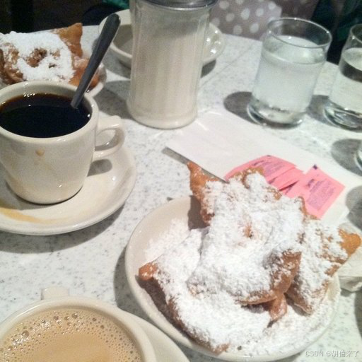
尝试使用`pipeline`对微调后的模型进行推理是最简单的方法。使用你的模型实例化一个图像分类的 pipeline,并将图像传递给它:
from transformers import pipeline

classifier = pipeline("image-classification", model="my_awesome_food_model")
classifier(image)
结果为:
[{'score': 0.31856709718704224, 'label': 'beignets'},
 {'score': 0.015232225880026817, 'label': 'bruschetta'},
 {'score': 0.01519392803311348, 'label': 'chicken_wings'},
 {'score': 0.013022331520915031, 'label': 'pork_chop'},
 {'score': 0.012728818692266941, 'label': 'prime_rib'}]
如果希望,你也可以手动复制 pipeline 的结果:
加载图像处理器对图像进行预处理,并将input返回为 PyTorch 张量:
from transformers import AutoImageProcessor
import torch

image_processor = AutoImageProcessor.from_pretrained("my_awesome_food_model")
inputs = image_processor(image, return_tensors="pt")
将输入传递给模型并返回 logits:
from transformers import AutoModelForImageClassification

model = AutoModelForImageClassification.from_pretrained("my_awesome_food_model")
with torch.no_grad():
     logits = model(**inputs).logits
使用最高概率的预测标签,并使用模型的 id2label 映射将其转换为标签:
predicted_label = logits.argmax(-1).item()
model.config.id2label[predicted_label]
结果为:
'beignets'加载图像处理器对图像进行预处理并将input返回为 TensorFlow 张量:
from transformers import AutoImageProcessor

image_processor = AutoImageProcessor.from_pretrained("MariaK/food_classifier")
inputs = image_processor(image, return_tensors="tf")
将输入传递给模型并返回 logits:
from transformers import TFAutoModelForImageClassification

model = TFAutoModelForImageClassification.from_pretrained("MariaK/food_classifier")
logits = model(**inputs).logits
使用最高概率的预测标签,并使用模型的 id2label 映射将其转换为标签:
predicted_class_id = int(tf.math.argmax(logits, axis=-1)[0])
model.config.id2label[predicted_class_id]
结果为:
'beignets'零样本图像分类
零样本图像分类(Zero-shot image classification)是一项用于既有分类还没有可用特征的模型上将图像划分类别的任务。
传统上,图像分类需要在一组既定的标签化图像上训练出的模型,这个模型学习将图像特征"映射"到标签上。当需要将这种模型用于引入到新的一组标签的分类任务时,需要微调以"重新校准"模型。
相比之下,零样本图像分类模型通常是在大量图像和相关描述数据集上训练的多模态模型。这些模型通过学习对齐的视觉语言表示,可用于许多下游任务,包括零采样图像分类。
这是一种更灵活的图像分类方法,它允许模型在不需要额外训练数据的情况下泛化到新的和未见过的类别,并使用户能够通过自由格式文本描述的图像信息查找具有目标对象图片。
在开始之前,请确保已安装所有必要的库:
pip install -q transformers零样本图像分类 pipeline
使用支持零样本图像分类的模型进行推断的最简单方法是使用 pipeline:
from transformers import pipeline

checkpoint = "openai/clip-vit-large-patch14"
detector = pipeline(model=checkpoint, task="zero-shot-image-classification")
接下来,选择要分类的图像。
from PIL import Image
import requests

url = "https://unsplash.com/photos/g8oS8-82DxI/download?ixid=MnwxMjA3fDB8MXx0b3BpY3x8SnBnNktpZGwtSGt8fHx8fDJ8fDE2NzgxMDYwODc&force=true&w=640"
image = Image.open(requests.get(url, stream=True).raw)

image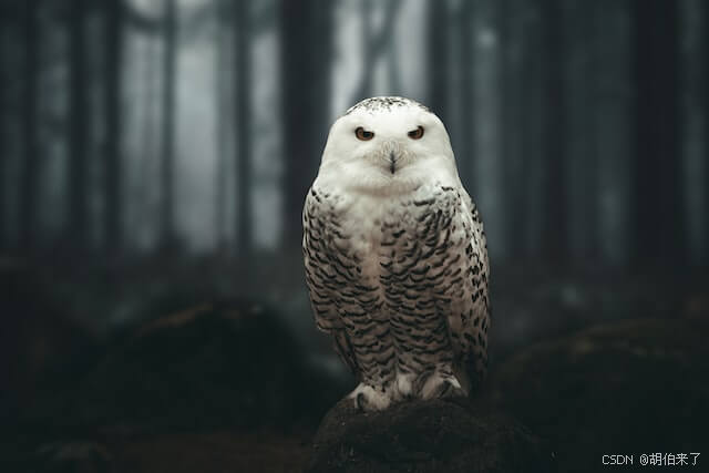
将图像和候选对象标签传递给 pipeline。在本示例中,我们直接传递图像;其他合适的选项包括图像的本地路径或图像的URL。 候选标签可以是简单的单词,就像这个示例中一样,也可以更详细描述。
predictions = detector(image, candidate_labels=["狐狸", "熊", "海鸥", "猫头鹰"])
predictions
结果:
[{'score': 0.9996670484542847, 'label': '猫头鹰'},
 {'score': 0.000199399160919711, 'label': '海鸥'},
 {'score': 7.392891711788252e-05, 'label': '狐狸'},
 {'score': 5.96074532950297e-05, 'label': '熊'}]
手动零样本图像分类
现在你已经了解了如何使用零样本图像分类流程,让我们来看看如何手动运行零样本图像分类。
from transformers import AutoProcessor, AutoModelForZeroShotImageClassification

model = AutoModelForZeroShotImageClassification.from_pretrained(checkpoint)
processor = AutoProcessor.from_pretrained(checkpoint)
我们来用一张不同的图片进行尝试。
from PIL import Image
import requests

url = "https://unsplash.com/photos/xBRQfR2bqNI/download?ixid=MnwxMjA3fDB8MXxhbGx8fHx8fHx8fHwxNjc4Mzg4ODEx&force=true&w=640"
image = Image.open(requests.get(url, stream=True).raw)

image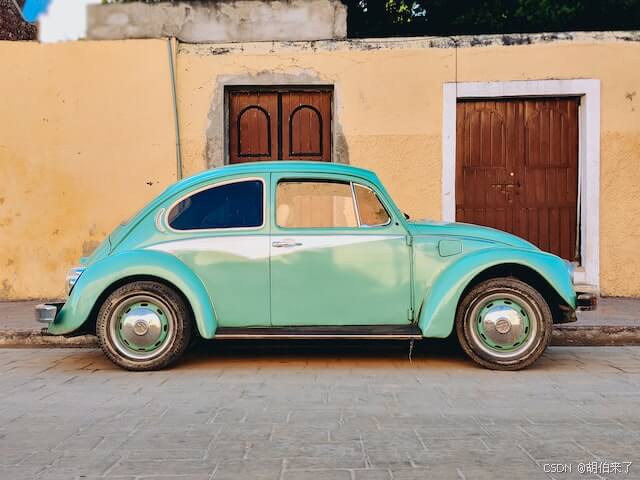
使用处理器为模型准备输入。处理器包括一个图像处理器,它通过调整大小和归一化来准备模型的图像,以及一个token处理器,它负责处理文本输入。
candidate_labels = ["树", "汽车", "自行车", "猫"]
inputs = processor(images=image, text=candidate_labels, return_tensors="pt", padding=True)
将输入传递给模型,并对结果进行后处理:
import torch

with torch.no_grad():
     outputs = model(**inputs)

logits = outputs.logits_per_image[0]
probs = logits.softmax(dim=-1).numpy()
scores = probs.tolist()

result = [
     {"score": score, "label": candidate_label}
     for score, candidate_label in sorted(zip(probs, candidate_labels), key=lambda x: -x[0])
 ]

result
结果:
[{'score': 0.998572, 'label': '汽车'},
 {'score': 0.0010570387, 'label': '自行车'},
 {'score': 0.0003393686, 'label': '树'},
 {'score': 3.1572064e-05, 'label': '猫'}]
图像转换
"图像到图像"(image-to-image)任务是应用程序接收图像并输出为另一个图像的任务。它有各种子任务,包括图像增强(超分辨率、低光照增强、去雾等)、图像修复等。
本章节技术点:
- 通过
pipeline调用image-to-image任务来完成超分辨率任务; - 直接调用
image-to-image特定任务类来完成。
首先先安装所需的依赖项:
pip install transformers我们现在可以在初始化 pipeline 时传入 Swin2SR 模型。然后,我们可以通过 pipeline 来推理。到目前为止,trasformers中只支持Swin2SR 模型。
from transformers import pipeline
import torch
from accelerate.test_utils.testing import get_backend

# automatically detects the underlying device type (CUDA, CPU, XPU, MPS, etc.)
device, _, _ = get_backend()
pipe = pipeline(task="image-to-image", model="caidas/swin2SR-lightweight-x2-64", device=device)
然后,我们加载图像:
from PIL import Image
import requests

url = "https://huggingface.co/datasets/huggingface/documentation-images/resolve/main/transformers/tasks/cat.jpg"
image = Image.open(requests.get(url, stream=True).raw)

print(image.size)
输出:
(532, 432)此时,我们通过pipeline执行推理,获取到高规格的新图片:
upscaled = pipe(image)
print(upscaled.size)
输出:
(1072, 880)如果不通过pipeline来加载 image-to-image 来进行推理,可以使用 transformer 的 Swin2SRForImageSuperResolution和Swin2SRImageProcessor 类。我们将初始化模型和处理器并使用相同的模型检查点。
from transformers import Swin2SRForImageSuperResolution, Swin2SRImageProcessor

model = Swin2SRForImageSuperResolution.from_pretrained("caidas/swin2SR-lightweight-x2-64").to(device)
processor = Swin2SRImageProcessor("caidas/swin2SR-lightweight-x2-64")pipeline封装了我们必须自己做的预处理和后处理步骤,现在我们只能自主对图像进行预处理。先将图像传递给处理器,然后将像素值移动到 GPU。
pixel_values = processor(image, return_tensors="pt").pixel_values
print(pixel_values.shape)

pixel_values = pixel_values.to(device)
将像素值传给模型后就可以对图像进行推理了:
import torch

with torch.no_grad():
  outputs = model(pixel_values)
输出的是 ImageSuperResolutionOutput 对象类型实例,结果类似:
(loss=None, reconstruction=tensor([[[[0.8270, 0.8269, 0.8275,  ..., 0.7463, 0.7446, 0.7453],
          [0.8287, 0.8278, 0.8283,  ..., 0.7451, 0.7448, 0.7457],
          [0.8280, 0.8273, 0.8269,  ..., 0.7447, 0.7446, 0.7452],
          ...,
          [0.5923, 0.5933, 0.5924,  ..., 0.0697, 0.0695, 0.0706],
          [0.5926, 0.5932, 0.5926,  ..., 0.0673, 0.0687, 0.0705],
          [0.5927, 0.5914, 0.5922,  ..., 0.0664, 0.0694, 0.0718]]]],
       device='cuda:0'), hidden_states=None, attentions=None)
我们需要重建并对其进行后处理以实现可视化。让我们看看它是什么样子的。
outputs.reconstruction.data.shape可视化数据如下:
torch.Size([1, 3, 880, 1072])我们需要压缩输出并删除轴0,裁剪值,然后将其转换为 numpy float。然后我们将坐标轴排列为形状1072,880,最后将输出恢复到范围0,255。
import numpy as np

# squeeze, take to CPU and clip the values
output = outputs.reconstruction.data.squeeze().cpu().clamp_(0, 1).numpy()
# rearrange the axes
output = np.moveaxis(output, source=0, destination=-1)
# bring values back to pixel values range
output = (output * 255.0).round().astype(np.uint8)
Image.fromarray(output)
图像分割
图像分割模型分离出图像中不同兴趣区域对应的区域。这些模型的工作原理是为每个像素分配一个标签。有几种类型的分割:语义分割、实例分割和全景分割。
在开始之前,请确保已安装所有必要的库:
pip install -q datasets transformers evaluate分割类型
图像分割种类包括语义分割 、实例分割 和全景分割等三种。
-
语义分割
语义分割为图像中的每个像素分配标签或类别。我们先看一看语义分割模型的输出:它将为图像中遇到的每个对象实例分配相同的类,例如,所有的猫将被标记为"cat",而不是"cat-1","cat-2"。
我们可以使用
transformer的图像分割管道来快速推断语义分割模型。让我们看一下示例。from transformers import pipeline from PIL import Image import requests url = "https://huggingface.co/datasets/huggingface/documentation-images/resolve/main/transformers/tasks/segmentation_input.jpg" image = Image.open(requests.get(url, stream=True).raw) image我们将使用
nvidia/segformer-b1-finetuned-cityscapes-1024-1024模型:semantic_segmentation = pipeline("image-segmentation", "nvidia/segformer-b1-finetuned-cityscapes-1024-1024") results = semantic_segmentation(image) results分割
pipeline输出包括每个预测类的掩码:[{'score': None, 'label': 'road', 'mask': <PIL.Image.Image image mode=L size=612x415>}, {'score': None, 'label': 'sidewalk', 'mask': <PIL.Image.Image image mode=L size=612x415>}, {'score': None, 'label': 'building', 'mask': <PIL.Image.Image image mode=L size=612x415>}, {'score': None, 'label': 'wall', 'mask': <PIL.Image.Image image mode=L size=612x415>}, {'score': None, 'label': 'pole', 'mask': <PIL.Image.Image image mode=L size=612x415>}, {'score': None, 'label': 'traffic sign', 'mask': <PIL.Image.Image image mode=L size=612x415>}, {'score': None, 'label': 'vegetation', 'mask': <PIL.Image.Image image mode=L size=612x415>}, {'score': None, 'label': 'terrain', 'mask': <PIL.Image.Image image mode=L size=612x415>}, {'score': None, 'label': 'sky', 'mask': <PIL.Image.Image image mode=L size=612x415>}, {'score': None, 'label': 'car', 'mask': <PIL.Image.Image image mode=L size=612x415>}]看一下
car类的掩码,我们可以看到每辆车都用同一个掩码类别。results[-1]["mask"] -
实例分割
在实例分割中,目标不是对每个像素进行分类,而是为给定图像中的每个对象实例 预测一个掩码。它的工作原理与对象检测非常相似,每个实例都有一个边界框,而不是一个分割掩码。我们将使用
facebook/mask2former-swin-large-cityscapes-instance来实现。instance_segmentation = pipeline("image-segmentation", "facebook/mask2former-swin-large-cityscapes-instance") results = instance_segmentation(image) results如下所示,有多辆汽车被分类,除了属于"car"和"person"实例的像素外,没有其他像素分类。
[{'score': 0.999944,
  'label': 'car',
  'mask': <PIL.Image.Image image mode=L size=612x415>},
 {'score': 0.999945,
  'label': 'car',
  'mask': <PIL.Image.Image image mode=L size=612x415>},
 {'score': 0.999652,
  'label': 'car',
  'mask': <PIL.Image.Image image mode=L size=612x415>},
 {'score': 0.903529,
  'label': 'person',
  'mask': <PIL.Image.Image image mode=L size=612x415>}]
看看下面的一个汽车面掩码。
results[2]["mask"] -
全景分割
全景分割结合了语义分割和实例分割,每个像素被分类到一个类和该类的一个实例中,每个类的实例都有多个掩码。我们可以使用
facebook/mask2former- sw-large -cityscape -panoptic。panoptic_segmentation = pipeline("image-segmentation", "facebook/mask2former-swin-large-cityscapes-panoptic") results = panoptic_segmentation(image) results结果如下所示(我们稍后将说明每个像素都被分类到其中一个类中):
[{'score': 0.999981,
  'label': 'car',
  'mask': <PIL.Image.Image image mode=L size=612x415>},
 {'score': 0.999958,
  'label': 'car',
  'mask': <PIL.Image.Image image mode=L size=612x415>},
 {'score': 0.99997,
  'label': 'vegetation',
  'mask': <PIL.Image.Image image mode=L size=612x415>},
 {'score': 0.999575,
  'label': 'pole',
  'mask': <PIL.Image.Image image mode=L size=612x415>},
 {'score': 0.999958,
  'label': 'building',
  'mask': <PIL.Image.Image image mode=L size=612x415>},
 {'score': 0.999634,
  'label': 'road',
  'mask': <PIL.Image.Image image mode=L size=612x415>},
 {'score': 0.996092,
  'label': 'sidewalk',
  'mask': <PIL.Image.Image image mode=L size=612x415>},
 {'score': 0.999221,
  'label': 'car',
  'mask': <PIL.Image.Image image mode=L size=612x415>},
 {'score': 0.99987,
  'label': 'sky',
  'mask': <PIL.Image.Image image mode=L size=612x415>}]
看到所有类型的切分,让我们深入了解语义切分模型的微调。
语义分割在现实世界中的常见应用包括训练自动驾驶汽车识别行人和重要的交通信息;识别医学图像中的细胞和异常;从卫星图像中监测环境变化等。
加载 SceneParse150 数据集
首先从数据集库中加载 SceneParse150 数据集的较小子集。在使用完整数据集进行更长时间的训练之前,这将为你提供实验和确保一切正常的机会。
from datasets import load_dataset

ds = load_dataset("scene_parse_150", split="train[:50]")使用`datasets.Dataset.train_test_split`方法将数据集的 train 拆分为训练集和测试集:
ds = ds.train_test_split(test_size=0.2)
train_ds = ds["train"]
test_ds = ds["test"]
然后查看一个示例:
train_ds[0]结果为:
{'image': <PIL.JpegImagePlugin.JpegImageFile image mode=RGB size=512x683 at 0x7F9B0C201F90>,
 'annotation': <PIL.PngImagePlugin.PngImageFile image mode=L size=512x683 at 0x7F9B0C201DD0>,
 'scene_category': 368}
其中:
image:场景的PIL图像。annotation:分割地图的PIL图像,也是模型的目标。scene_category:描述图像场景的类别ID,如kitchen或office。在本指南中,你只需要image和annotation,它们都是PIL图像。
你还需要创建一个字典,将 标签id 映射到 标签类别,这在设置模型时将很有用。从Hub下载映射并创建 id2label 和 label2id 字典:
import json
from huggingface_hub import cached_download, hf_hub_url

repo_id = "huggingface/label-files"
filename = "ade20k-id2label.json"
id2label = json.load(open(cached_download(hf_hub_url(repo_id, filename, repo_type="dataset")), "r"))
id2label = {int(k): v for k, v in id2label.items()}
label2id = {v: k for k, v in id2label.items()}
num_labels = len(id2label)
预处理
下一步是加载 SegFormer 图像处理器,以准备图像和注释供模型使用。一些数据集(例如此数据集)使用零索引作为背景类别。但是,实际上背景类别不包括在这150个类别中,因此你需要设置 reduce_labels=True,将所有标签减1。零索引由255替换,因此 SegFormer 的损失函数会忽略它:
from transformers import AutoImageProcessor

checkpoint = "nvidia/mit-b0"
image_processor = AutoImageProcessor.from_pretrained(checkpoint, reduce_labels=True)
通常在图像数据集上应用一些数据增强方法,以使模型对过拟合更具鲁棒性。在本指南中,你将使用 ColorJitter 函数,随机更改图像的颜色属性,但你也可以使用你喜欢的任何图像库。
from torchvision.transforms import ColorJitter

jitter = ColorJitter(brightness=0.25, contrast=0.25, saturation=0.25, hue=0.1)
现在创建两个预处理函数,以准备图像和注释供模型使用。这些函数将图像转换为 pixel_values,将注释转换为 labels。对于训练集,在将图像提供给图像处理器之前,应用 jitter。对于测试集,图像处理器对 images 进行裁剪和归一化,只裁剪 labels,因为在测试期间不应用数据增强。
def train_transforms(example_batch):
     images = [jitter(x) for x in example_batch["image"]]
     labels = [x for x in example_batch["annotation"]]
     inputs = image_processor(images, labels)
     return inputs

def val_transforms(example_batch):
     images = [x for x in example_batch["image"]]
     labels = [x for x in example_batch["annotation"]]
     inputs = image_processor(images, labels)
return inputs使用数据集`datasets.Dataset.set_transform`函数在整个数据集上应用 jitter。变换是即时应用的,速度更快,占用的磁盘空间更少:
train_ds.set_transform(train_transforms)
test_ds.set_transform(val_transforms)
通常,在图像数据集上应用一些数据增强方法可以提高模型对过拟合的鲁棒性。 在本指南中,你将使用 tf.image 随机更改图像的颜色属性,但你也可以使用你喜欢的任何图像库。 请定义两个不同的转换函数:
-
包含图像增强的训练数据转换
-
仅转置图像的验证数据转换,因为
Transformers中的计算机视觉模型需要以通道优先的布局(channels-first layout)import tensorflow as tf
def aug_transforms(image):
image = tf.keras.utils.img_to_array(image)
image = tf.image.random_brightness(image, 0.25)
image = tf.image.random_contrast(image, 0.5, 2.0)
image = tf.image.random_saturation(image, 0.75, 1.25)
image = tf.image.random_hue(image, 0.1)
image = tf.transpose(image, (2, 0, 1))
return imagedef transforms(image):
image = tf.keras.utils.img_to_array(image)
image = tf.transpose(image, (2, 0, 1))
return image
接下来,创建两个预处理函数,以准备图像和注释的批次供模型使用。这些函数应用图像转换,并使用之前加载的 image_processor 将图像转换为 pixel_values 和注释转换为 labels。ImageProcessor 还负责调整大小和归一化图像。
def train_transforms(example_batch):
     images = [aug_transforms(x.convert("RGB")) for x in example_batch["image"]]
     labels = [x for x in example_batch["annotation"]]
     inputs = image_processor(images, labels)
     return inputs

def val_transforms(example_batch):
     images = [transforms(x.convert("RGB")) for x in example_batch["image"]]
     labels = [x for x in example_batch["annotation"]]
     inputs = image_processor(images, labels)
return inputs使用数据集`datasets.Dataset.set_transform`函数在整个数据集上应用预处理转换。变换是即时应用的,速度更快,占用的磁盘空间更少:
train_ds.set_transform(train_transforms)
test_ds.set_transform(val_transforms)
评估
在训练过程中包含一个度量指标通常有助于评估模型的性能。你可以使用 Evaluate 库快速加载一个评估方法。对于此任务,加载 mean Intersection over Union(IoU)度量指标:
import evaluate

metric = evaluate.load("mean_iou")然后创建一个函数来`evaluate.EvaluationModule.compute`度量指标。首先需要将预测转换为 logits,然后将其重塑为与标签大小相匹配,然后才能调用`evaluate.EvaluationModule.compute`:
import numpy as np
import torch
from torch import nn

def compute_metrics(eval_pred):
     with torch.no_grad():
         logits, labels = eval_pred
         logits_tensor = torch.from_numpy(logits)
         logits_tensor = nn.functional.interpolate(
             logits_tensor,
             size=labels.shape[-2:],
             mode="bilinear",
             align_corners=False,
         ).argmax(dim=1)

         pred_labels = logits_tensor.detach().cpu().numpy()
         metrics = metric.compute(
             predictions=pred_labels,
             references=labels,
             num_labels=num_labels,
             ignore_index=255,
             reduce_labels=False,
         )
         for key, value in metrics.items():
             if type(value) is np.ndarray:
                 metrics[key] = value.tolist()
         return metrics

def compute_metrics(eval_pred):
     logits, labels = eval_pred
     logits = tf.transpose(logits, perm=[0, 2, 3, 1])
     logits_resized = tf.image.resize(
         logits,
         size=tf.shape(labels)[1:],
         method="bilinear",
     )

     pred_labels = tf.argmax(logits_resized, axis=-1)
     metrics = metric.compute(
         predictions=pred_labels,
         references=labels,
         num_labels=num_labels,
         ignore_index=-1,
         reduce_labels=image_processor.do_reduce_labels,
     )

     per_category_accuracy = metrics.pop("per_category_accuracy").tolist()
     per_category_iou = metrics.pop("per_category_iou").tolist()

     metrics.update({f"accuracy_{id2label[i]}": v for i, v in enumerate(per_category_accuracy)})
     metrics.update({f"iou_{id2label[i]}": v for i, v in enumerate(per_category_iou)})
     return {"val_" + k: v for k, v in metrics.items()}
现在你的 compute_metrics 函数已准备就绪,请在设置训练时返回。
训练
现在可以开始训练模型了!使用`AutoModelForSemanticSegmentation`加载 SegFormer,并将模型与 标签id 和 标签类别 之间的映射传递给模型:
from transformers import AutoModelForSemanticSegmentation, TrainingArguments, Trainer

model = AutoModelForSemanticSegmentation.from_pretrained(checkpoint, id2label=id2label, label2id=label2id)
此时,只剩下三个步骤:
-
在`TrainingArguments`中定义训练超参数。重要的是不要删除未使用的列,因为这将删除
image列。没有image列,你无法创建pixel_values。将remove_unused_columns=False设置为防止此行为!仅其他必需的参数是output_dir,它指定保存模型的位置。设置push_to_hub=True将此模型推送到Hub(需要登录Hugging Face以上传你的模型)。在每个epoch结束时,`Trainer`将评估IoU度量并保存训练检查点。 -
将训练参数以及模型、数据集、
tokenizer、数据收集器和compute_metrics函数传递给`Trainer`。 -
调用`Trainer.train`开始微调模型。
training_args = TrainingArguments(
output_dir="segformer-b0-scene-parse-150",
learning_rate=6e-5,
num_train_epochs=50,
per_device_train_batch_size=2,
per_device_eval_batch_size=2,
save_total_limit=3,
evaluation_strategy="steps",
save_strategy="steps",
save_steps=20,
eval_steps=20,
logging_steps=1,
eval_accumulation_steps=5,
remove_unused_columns=False,
push_to_hub=True,
)trainer = Trainer(
model=model,
args=training_args,
train_dataset=train_ds,
eval_dataset=test_ds,
compute_metrics=compute_metrics,
)trainer.train()
完成训练后,请使用`transformers.Trainer.push_to_hub`方法将模型分享到Hub,以便每个人都可以使用你的模型:
trainer.push_to_hub()要在 TensorFlow 中微调模型,请按照以下步骤进行:
-
定义训练超参数,并设置优化器和学习率计划。
-
实例化预训练模型。
-
将数据集转换为
tf.data.Dataset。 -
编译模型。
-
添加回调函数来计算指标和上传模型到Hub。
-
使用fit()方法来运行训练。
步骤1:定义训练超参数
learning_rate = tf.keras.optimizers.schedules.PiecewiseConstantDecay(
boundaries=[100, 300, 500, 1000, 3000],
values=[1e-4, 5e-5, 3e-5, 1e-5, 1e-6, 1e-7])步骤2:实例化预训练模型
model = AutoModelForSemanticSegmentation.from_pretrained(checkpoint, id2label=id2label, label2id=label2id)
步骤3:将Dataset转换为
tf.data.Datasettrain_dataset = train_ds.to_tf_dataset(with_transform=train_transforms)
步骤4:编译模型
optimizer = tf.keras.optimizers.Adam(learning_rate=learning_rate)
model.compile(optimizer=optimizer)步骤5:添加回调函数
checkpoint_callback = tf.keras.callbacks.ModelCheckpoint(
filepath="checkpoint.h5",
save_weights_only=True,
save_best_only=True,
monitor="val_loss",
mode="min",
)步骤6:使用
fit()方法进行训练model.fit(
train_dataset,
validation_data=test_ds,
epochs=50,
callbacks=[checkpoint_callback],
)步骤7:将模型保存到Hub
model.save_pretrained("segformer-b0-scene-parse-150-tf")
推理
既然你已经微调了模型,那么可以用它进行推理!
加载用于推理的图像:
image = ds[0]["image"]
image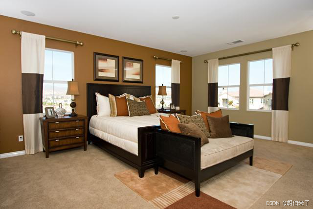
尝试使用模型进行推理的最简单的方法是使用`pipeline`。使用模型实例化一个图像分割的pipeline,然后将图像传递给它:
from transformers import pipeline

segmenter = pipeline("image-segmentation", model="my_awesome_seg_model")
segmenter(image)
结果为:
[{'score': None,
  'label': 'wall',
  'mask': <PIL.Image.Image image mode=L size=640x427 at 0x7FD5B2062690>},
 {'score': None,
  'label': 'sky',
  'mask': <PIL.Image.Image image mode=L size=640x427 at 0x7FD5B2062A50>},
 {'score': None,
  'label': 'floor',
  'mask': <PIL.Image.Image image mode=L size=640x427 at 0x7FD5B2062B50>},
 {'score': None,
  'label': 'ceiling',
  'mask': <PIL.Image.Image image mode=L size=640x427 at 0x7FD5B2062A10>},
 {'score': None,
  'label': 'bed ',
  'mask': <PIL.Image.Image image mode=L size=640x427 at 0x7FD5B2062E90>},
 {'score': None,
  'label': 'windowpane',
  'mask': <PIL.Image.Image image mode=L size=640x427 at 0x7FD5B2062390>},
 {'score': None,
  'label': 'cabinet',
  'mask': <PIL.Image.Image image mode=L size=640x427 at 0x7FD5B2062550>},
 {'score': None,
  'label': 'chair',
  'mask': <PIL.Image.Image image mode=L size=640x427 at 0x7FD5B2062D90>},
 {'score': None,
  'label': 'armchair',
  'mask': <PIL.Image.Image image mode=L size=640x427 at 0x7FD5B2062E10>}]
如果需要,你还可以手动复制 pipeline 的结果。使用图像处理器处理图像,并将 pixel_values 放在GPU上:
device = torch.device("cuda" if torch.cuda.is_available() else "cpu")  # 如果有可用的GPU,则使用GPU,否则使用CPU
encoding = image_processor(image, return_tensors="pt")
pixel_values = encoding.pixel_values.to(device)
将输入传递给模型并返回 logits:
outputs = model(pixel_values=pixel_values)
logits = outputs.logits.cpu()
接下来,将 logits 调整到原始图像的大小:
upsampled_logits = nn.functional.interpolate(
    logits,
    size=image.size[::-1],
    mode="bilinear",
    align_corners=False,
)

pred_seg = upsampled_logits.argmax(dim=1)[0]
加载图像处理器以预处理图像并以 TensorFlow 张量的形式返回输入:
from transformers import AutoImageProcessor

image_processor = AutoImageProcessor.from_pretrained("MariaK/scene_segmentation")
inputs = image_processor(image, return_tensors="tf")
将输入传递给模型并返回 logits:
from transformers import TFAutoModelForSemanticSegmentation

model = TFAutoModelForSemanticSegmentation.from_pretrained("MariaK/scene_segmentation")
logits = model(**inputs).logits
接下来,将 logits 调整到原始图像的大小,并对类维度应用 argmax 函数:
logits = tf.transpose(logits, [0, 2, 3, 1])

upsampled_logits = tf.image.resize(
    logits,
    # 由于`image.size`返回宽度和高度,所以我们颠倒了`image`的形状。
    image.size[::-1],
)

pred_seg = tf.math.argmax(upsampled_logits, axis=-1)[0]要可视化结果,加载数据集颜色调色板作为 ade_palette() 将每个类别映射到RGB值。然后,你可以将图像和预测的分割图组合在一起并绘制出来:
import matplotlib.pyplot as plt
import numpy as np

color_seg = np.zeros((pred_seg.shape[0], pred_seg.shape[1], 3), dtype=np.uint8)
palette = np.array(ade_palette())
for label, color in enumerate(palette):
    color_seg[pred_seg == label, :] = color
color_seg = color_seg[..., ::-1]  # 转换为BGR

img = np.array(image) * 0.5 + color_seg * 0.5  # 将图像与分割图重叠显示
img = img.astype(np.uint8)

plt.figure(figsize=(15, 10))
plt.imshow(img)
plt.show()
Image of bedroom overlaid with segmentation map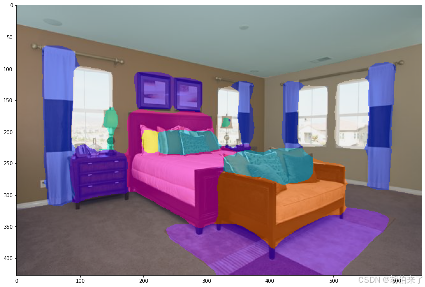
图像特征提取
图像特征提取是指从给定的图像中提取有语义意义的特征;这有很多用例如"图像相似性"和"图像检索"等。此外,大多数计算机视觉模型可以用于图像特征提取,其中之一可以删除特定任务的头部(图像分类、目标检测等)并获得特征。这些特征在更高层次的应用(如边缘检测、角点检测等)上非常有用。它们还可能包含关于现实世界的信息(例如,猫看起来像什么),这取决于模型的深度。因此,这些输出可用于在特定数据集上训练新的分类器。
在本节中,你将:
- 学会在"图像-特征-提取"管道之上构建一个简单的图像相似性系统。
- 使用裸模型推理完成相同的任务。
使用 image-feature-extraction 任务判断图像相似度
我们有两张猫坐在渔网上的图像,其中一张是生成的:
from PIL import Image
import requests

img_urls = ["https://huggingface.co/datasets/huggingface/documentation-images/resolve/main/cats.png", "https://huggingface.co/datasets/huggingface/documentation-images/resolve/main/cats.jpeg"]
image_real = Image.open(requests.get(img_urls[0], stream=True).raw).convert("RGB")
image_gen = Image.open(requests.get(img_urls[1], stream=True).raw).convert("RGB")
让我们看看 pipeline 任务处理的实际效果。首先,初始化 pipeline 并设定使用的任务为 image-feature-extraction。如果您不传递任何模型给它,pipeline 将自动初始化 goolge/vit-base-patch16-224。如果你想计算相似度,将pool设置为 True:
import torch
from transformers import pipeline
from accelerate.test_utils.testing import get_backend
# automatically detects the underlying device type (CUDA, CPU, XPU, MPS, etc.)
DEVICE, _, _ = get_backend()
pipe = pipeline(task="image-feature-extraction", model_name="google/vit-base-patch16-384", device=DEVICE, pool=True)
然后通过 pipe传入两张图片做比较:
outputs = pipe([image_real, image_gen])输出包含这两个图像的池化嵌入。
# get the length of a single output
print(len(outputs[0][0]))
# show outputs
print(outputs)
打印结果:
768
[[[-0.03909236937761307, 0.43381670117378235, -0.06913255900144577,如果你想在池化之前获取最后的隐藏状态,请避免通过pool参数传入任何值,因为该参数默认False。这些隐藏状态对于基于模型特征训练新的分类器或模型非常有用。
pipe = pipeline(task="image-feature-extraction", model_name="google/vit-base-patch16-224", device=DEVICE)
outputs = pipe(image_real)
由于输出是未池化的,我们得到最后的隐藏状态:其中第一个维度是批量大小,最后两个是嵌入形状。
import numpy as np
print(np.array(outputs).shape)
输出:
(1, 197, 768)使用 AutoModel获取特征和相似度
我们也可以使用 transformer 的Automdel类来获取特征。Automdel 加载任何没有特定任务头的 transformer 模型,我们可以使用它来获取特征。
from transformers import AutoImageProcessor, AutoModel

processor = AutoImageProcessor.from_pretrained("google/vit-base-patch16-224")
model = AutoModel.from_pretrained("google/vit-base-patch16-224").to(DEVICE)让我们写一个简单的函数来进行推断。我们将首先将输入传递给processor,并将其输出传递给model。
def infer(image):
  inputs = processor(image, return_tensors="pt").to(DEVICE)
  outputs = model(**inputs)
  return outputs.pooler_output
我们可以直接将图像传递给这个函数并获得嵌入。
embed_real = infer(image_real)
embed_gen = infer(image_gen)
我们可以通过嵌入再次得到相似度。
from torch.nn.functional import cosine_similarity

similarity_score = cosine_similarity(embed_real, embed_gen, dim=1)
print(similarity_score)
输出:
tensor([0.6061], device='cuda:0', grad_fn=<SumBackward1>)关键点检测
关键点检测识别并定位图像中特定的感兴趣的点。这些关键点也称为"路标",表示物体的有意义的特征,如面部特征或物体部位。这些模型接受一个图像输入,并返回以下输出:
- 关键点和得分:兴趣点及其置信度得分。
- 描述符:表示每个关键点周围的图像区域,捕捉其纹理、梯度、方向和其他属性。
在本节中,我们利用 SuperPoint 来展示如何从图像中提取关键点:
from transformers import AutoImageProcessor, SuperPointForKeypointDetection
processor = AutoImageProcessor.from_pretrained("magic-leap-community/superpoint")
model = SuperPointForKeypointDetection.from_pretrained("magic-leap-community/superpoint")
现在,我们通过一张图来测试模型:
import torch
from PIL import Image
import requests
import cv2


url_image_1 = "https://huggingface.co/datasets/huggingface/documentation-images/resolve/main/bee.jpg"
image_1 = Image.open(requests.get(url_image_1, stream=True).raw)
url_image_2 = "https://huggingface.co/datasets/huggingface/documentation-images/resolve/main/cats.png"
image_2 = Image.open(requests.get(url_image_2, stream=True).raw)

images = [image_1, image_2]
接下来开始处理输入并推断:
inputs = processor(images,return_tensors="pt").to(model.device, model.dtype)
outputs = model(**inputs)
模型输出具有批处理中每个项目的相对关键点、描述符、掩码和分数。蒙版突出显示图像中存在关键点的区域。
SuperPointKeypointDescriptionOutput(loss=None, keypoints=tensor([[[0.0437, 0.0167],
         [0.0688, 0.0167],
         [0.0172, 0.0188],
         ...,
         [0.5984, 0.9812],
         [0.6953, 0.9812]]]),
         scores=tensor([[0.0056, 0.0053, 0.0079,  ..., 0.0125, 0.0539, 0.0377],
        [0.0206, 0.0058, 0.0065,  ..., 0.0000, 0.0000, 0.0000]],
       grad_fn=<CopySlices>), descriptors=tensor([[[-0.0807,  0.0114, -0.1210,  ..., -0.1122,  0.0899,  0.0357],
         [-0.0807,  0.0114, -0.1210,  ..., -0.1122,  0.0899,  0.0357],
         [-0.0807,  0.0114, -0.1210,  ..., -0.1122,  0.0899,  0.0357],
         ...],
       grad_fn=<CopySlices>), mask=tensor([[1, 1, 1,  ..., 1, 1, 1],
[1, 1, 1, ..., 0, 0, 0]], dtype=torch.int32), hidden_states=None)为了在图像中绘制实际的关键点,我们需要对输出进行后处理。为此,我们必须将实际图像大小和输出一起传给post_process_keypoint_detection。
image_sizes = [(image.size[1], image.size[0]) for image in images]
outputs = processor.post_process_keypoint_detection(outputs, image_sizes)
输出现在是一个字典列表,其中每个字典都是关键点、分数和描述符的处理后输出。
[{'keypoints': tensor([[ 226,   57],
          [ 356,   57],
          [  89,   64],
          ...,
          [3604, 3391]], dtype=torch.int32),
  'scores': tensor([0.0056, 0.0053, ...], grad_fn=<IndexBackward0>),
  'descriptors': tensor([[-0.0807,  0.0114, -0.1210,  ..., -0.1122,  0.0899,  0.0357],
          [-0.0807,  0.0114, -0.1210,  ..., -0.1122,  0.0899,  0.0357]],
         grad_fn=<IndexBackward0>)},
    {'keypoints': tensor([[ 46,   6],
          [ 78,   6],
          [422,   6],
          [206, 404]], dtype=torch.int32),
  'scores': tensor([0.0206, 0.0058, 0.0065, 0.0053, 0.0070, ...,grad_fn=<IndexBackward0>),
  'descriptors': tensor([[-0.0525,  0.0726,  0.0270,  ...,  0.0389, -0.0189, -0.0211],
          [-0.0525,  0.0726,  0.0270,  ...,  0.0389, -0.0189, -0.0211]}]
我们利用这些关键点来绘制:
import matplotlib.pyplot as plt
import torch

for i in range(len(images)):
  keypoints = outputs[i]["keypoints"]
  scores = outputs[i]["scores"]
  descriptors = outputs[i]["descriptors"]
  keypoints = outputs[i]["keypoints"].detach().numpy()
  scores = outputs[i]["scores"].detach().numpy()
  image = images[i]
  image_width, image_height = image.size

  plt.axis('off')
  plt.imshow(image)
  plt.scatter(
      keypoints[:, 0],
      keypoints[:, 1],
      s=scores * 100,
      c='cyan',
      alpha=0.4
  )
  plt.show()
目标检测
目标检测是计算机视觉的任务之一,用于在图像中检测实例(例如人、建筑物或汽车等)。目标检测模型接收图像作为输入,并输出检测到的对象的边界框的坐标和关联标签。一张图像可以包含多个对象,每个对象都有自己的边界框和标签(例如可以同时包含汽车和建筑物),每个对象可以出现在图像的不同部分(例如图像中可能有几辆汽车)。这个任务在自动驾驶中常用于检测像行人、道路标志和交通灯等物体。其他应用包括图像中对象计数、图像搜索等。
任务支持以下模型架构:
Conditional DETR, Deformable DETR, DETA, DETR, Table Transformer, YOLOS
在开始之前,请确保已安装所有必要的库:
pip install -q datasets transformers evaluate timm albumentations加载 CPPE-5 数据集
CPPE-5 数据集 包含在 COVID-19 疫情背景下识别医疗个人防护装备(PPE)的图像。
首先加载数据集:
from datasets import load_dataset

cppe5 = load_dataset("cppe-5")
cppe5
结果:
DatasetDict({
    train: Dataset({
        features: ['image_id', 'image', 'width', 'height', 'objects'],
        num_rows: 1000
    })
    test: Dataset({
        features: ['image_id', 'image', 'width', 'height', 'objects'],
        num_rows: 29
    })
})
你会发现这个数据集已经包含了一个包含 1000 张图像的训练集和一个包含 29 张图像的测试集。
为了熟悉数据,查看一下示例的样子。
cppe5["train"][0]结果:
{'image_id': 15,
 'image': <PIL.JpegImagePlugin.JpegImageFile image mode=RGB size=943x663 at 0x7F9EC9E77C10>,
 'width': 943,
 'height': 663,
 'objects': {'id': [114, 115, 116, 117],
  'area': [3796, 1596, 152768, 81002],
  'bbox': [[302.0, 109.0, 73.0, 52.0],
   [810.0, 100.0, 57.0, 28.0],
   [160.0, 31.0, 248.0, 616.0],
   [741.0, 68.0, 202.0, 401.0]],
  'category': [4, 4, 0, 0]}}
数据集中的示例包括以下字段:
image_id:示例图像的IDimageV:包含图像的 PIL.Image.Image 对象 Vwidth:图像的宽度height:图像的高度objects:包含图像中对象的边界框元数据的字典:id:注释的 IDarea:边界框的面积bbox:对象的边界框(COCO 格式)category:对象的类别,可能的值包括Coverall(0)、Face_Shield(1)、Gloves(2)、Goggles(3) 或Mask(4)
你可能会注意到 bbox 字段遵循 COCO 格式,这是 DETR 模型希望的格式。 然而,objects 中字段的分组与 DETR 要求的注释格式不同。你需要在使用此数据进行训练之前应用一些预处理转换。
为了更好地了解数据,可视化数据集中的一个示例。
import numpy as np
import os
from PIL import Image, ImageDraw

image = cppe5["train"][0]["image"]
annotations = cppe5["train"][0]["objects"]
draw = ImageDraw.Draw(image)

categories = cppe5["train"].features["objects"].feature["category"].names

id2label = {index: x for index, x in enumerate(categories, start=0)}
label2id = {v: k for k, v in id2label.items()}

for i in range(len(annotations["id"])):
     box = annotations["bbox"][i - 1]
     class_idx = annotations["category"][i - 1]
     x, y, w, h = tuple(box)
     draw.rectangle((x, y, x + w, y + h), outline="red", width=1)
     draw.text((x, y), id2label[class_idx], fill="white")

image
结果:
要可视化带有关联标签的边界框,你可以从数据集的元数据中获取标签,特别是 category 字段。 你还需要创建映射将标签 ID 映射到标签类别(id2label),以及将标签类别映射到 ID 的映射(label2id)。 如果你在 Hugging Face Hub 上分享模型,包括这些映射将使你的模型可以被其他人重复使用。
在了解数据的过程中,要侧重检查潜在问题。对象检测数据集中的一个常见问题是边界框"拉伸"到图像边缘以外。这样的"行为"边界框可能会在训练时引发错误,并且应该在此阶段予以解决。在此数据集中有几个示例存在这个问题。为了简化本指南,我们从数据中删除这些图像。
remove_idx = [590, 821, 822, 875, 876, 878, 879]
keep = [i for i in range(len(cppe5["train"])) if i not in remove_idx]
cppe5["train"] = cppe5["train"].select(keep)
对数据进行预处理
要微调模型,你必须预处理计划使用的数据,以精确地匹配预训练模型所使用的方法。 `AutoImageProcessor` 负责处理图像数据,创建 pixel_values、pixel_mask 和可以用于训练 DETR 模型的 labels。图像处理器具有一些你不必担心的属性:
image_mean = [0.485, 0.456, 0.406]
image_std = [0.229, 0.224, 0.225]
这些是用于规范化模型在预训练期间的图像的平均值和标准差。当进行推断或微调预训练图像模型时,这些值非常重要。
从与预处理使用的检查点相同的检查点实例化图像处理器。
from transformers import AutoImageProcessor

checkpoint = "facebook/detr-resnet-50"
image_processor = AutoImageProcessor.from_pretrained(checkpoint)
在将图像传递给 image_processor 之前,应用两种预处理转换对数据集进行预处理:
- 对图像进行增强
- 重新格式化注释以满足 DETR 的预期
首先,为了确保模型不会过度拟合训练数据,可以使用任何数据增强库对图像进行增强。这里我们使用 Albumentations... 该库确保转换影响图像并相应地更新边界框。Datasets 库的文档中有一个详细的 关于如何为对象检测增强图像的指南,它使用完全相同的数据集作为示例。在这里应用相同的方法,将每个图像调整为 (480, 480) 的大小,水平翻转图像,并增加亮度:
import albumentations
import numpy as np
import torch

transform = albumentations.Compose(
     [
         albumentations.Resize(480, 480),
         albumentations.HorizontalFlip(p=1.0),
         albumentations.RandomBrightnessContrast(p=1.0),
     ],
     bbox_params=albumentations.BboxParams(format="coco", label_fields=["category"]),
 )
image_processor 期望注释的格式为:{'image_id': int, 'annotations': List[Dict]},其中每个字典都是 COCO 对象注释。让我们添加一个函数,以重新格式化单个示例的注释:
def formatted_anns(image_id, category, area, bbox):
     annotations = []
     for i in range(0, len(category)):
         new_ann = {
             "image_id": image_id,
             "category_id": category[i],
             "isCrowd": 0,
             "area": area[i],
             "bbox": list(bbox[i]),
         }
         annotations.append(new_ann)

     return annotations
现在,你可以将图像和注释转换组合起来以在一批示例上使用:
# transforming a batch
def transform_aug_ann(examples):
     image_ids = examples["image_id"]
     images, bboxes, area, categories = [], [], [], []
     for image, objects in zip(examples["image"], examples["objects"]):
         image = np.array(image.convert("RGB"))[:, :, ::-1]
         out = transform(image=image, bboxes=objects["bbox"], category=objects["category"])

         area.append(objects["area"])
         images.append(out["image"])
         bboxes.append(out["bboxes"])
         categories.append(out["category"])

     targets = [
         {"image_id": id_, "annotations": formatted_anns(id_, cat_, ar_, box_)}
         for id_, cat_, ar_, box_ in zip(image_ids, categories, area, bboxes)
     ]

     return image_processor(images=images, annotations=targets, return_tensors="pt")
使用 Datasets 的 `datasets.Dataset.with_transform` 方法将此预处理函数应用于整个数据集。此方法在加载数据集元素时动态应用转换。
此时,你可以检查经过转换的数据集中的示例的样子了。你应该会看到带有 pixel_values 的张量,带有 pixel_mask 的张量和 labels。
cppe5["train"] = cppe5["train"].with_transform(transform_aug_ann)
cppe5["train"][15]
结果为:
{'pixel_values': tensor([[[ 0.9132,  0.9132,  0.9132,  ..., -1.9809, -1.9809, -1.9809],
          [ 0.9132,  0.9132,  0.9132,  ..., -1.9809, -1.9809, -1.9809],
          [ 0.9132,  0.9132,  0.9132,  ..., -1.9638, -1.9638, -1.9638],
          ...,
          [-1.5699, -1.5699, -1.5699,  ..., -1.9980, -1.9980, -1.9980],
          [-1.5528, -1.5528, -1.5528,  ..., -1.9980, -1.9809, -1.9809],
          [-1.5528, -1.5528, -1.5528,  ..., -1.9980, -1.9809, -1.9809]],

         [[ 1.3081,  1.3081,  1.3081,  ..., -1.8431, -1.8431, -1.8431],
          [ 1.3081,  1.3081,  1.3081,  ..., -1.8431, -1.8431, -1.8431],
          [ 1.3081,  1.3081,  1.3081,  ..., -1.8256, -1.8256, -1.8256],
          ...,
          [-1.3179, -1.3179, -1.3179,  ..., -1.8606, -1.8606, -1.8606],
          [-1.3004, -1.3004, -1.3004,  ..., -1.8606, -1.8431, -1.8431],
          [-1.3004, -1.3004, -1.3004,  ..., -1.8606, -1.8431, -1.8431]],

         [[ 1.4200,  1.4200,  1.4200,  ..., -1.6476, -1.6476, -1.6476],
          [ 1.4200,  1.4200,  1.4200,  ..., -1.6476, -1.6476, -1.6476],
          [ 1.4200,  1.4200,  1.4200,  ..., -1.6302, -1.6302, -1.6302],
          ...,
          [-1.0201, -1.0201, -1.0201,  ..., -1.5604, -1.5604, -1.5604],
          [-1.0027, -1.0027, -1.0027,  ..., -1.5604, -1.5430, -1.5430],
          [-1.0027, -1.0027, -1.0027,  ..., -1.5604, -1.5430, -1.5430]]]),
 'pixel_mask': tensor([[1, 1, 1,  ..., 1, 1, 1],
         [1, 1, 1,  ..., 1, 1, 1],
         [1, 1, 1,  ..., 1, 1, 1],
         ...,
         [1, 1, 1,  ..., 1, 1, 1],
         [1, 1, 1,  ..., 1, 1, 1],
         [1, 1, 1,  ..., 1, 1, 1]]),
 'labels': {'size': tensor([800, 800]), 'image_id': tensor([756]), 'class_labels': tensor([4]), 'boxes': tensor([[0.7340, 0.6986, 0.3414, 0.5944]]), 'area': tensor([519544.4375]), 'iscrowd': tensor([0]), 'orig_size': tensor([480, 480])}}
你已成功增强了个别图像并准备了它们的注释。然而,预处理还没有完成。在最后一步中,创建一个自定义的 collate_fn 来将图像批处理在一起。 将图像(现在是 pixel_values)填充到一批中最大的图像,创建相应的 pixel_mask 来指示哪些像素是真实的(1)和哪些是填充的(0)。
def collate_fn(batch):
     pixel_values = [item["pixel_values"] for item in batch]
     encoding = image_processor.pad(pixel_values, return_tensors="pt")
     labels = [item["labels"] for item in batch]
     batch = {}
     batch["pixel_values"] = encoding["pixel_values"]
     batch["pixel_mask"] = encoding["pixel_mask"]
     batch["labels"] = labels
     return batch
训练 DEER 模型
在之前的部分中,你已经完成了大部分繁重的工作,现在可以开始训练模型了!即使在调整大小之后,此数据集中的图像仍然相当大。这意味着微调此模型将需要至少一个 GPU。
训练包括以下步骤:
- 使用与预处理相同的检查点使用 `AutoModelForObjectDetection` 加载模型。
- 在 `TrainingArguments` 中定义你的训练超参数。
- 将训练参数与模型、数据集、图像处理器和数据收集器一起传递给 `Trainer`。
- 调用 `Trainer.train` 来微调你的模型。
在从与预处理相同的检查点加载模型时,请记得传递之前从数据集的元数据中创建的 label2id 和 id2label 映射。此外,我们指定了 ignore_mismatched_sizes=True 来用新的分类头替换现有的分类头。
from transformers import AutoModelForObjectDetection

model = AutoModelForObjectDetection.from_pretrained(
     checkpoint,
     id2label=id2label,
     label2id=label2id,
     ignore_mismatched_sizes=True,
 )
在 `TrainingArguments` 中,使用 output_dir 指定保存模型的位置,然后根据需要配置超参数。请务必不要删除未使用的列,因为这会丢弃 image 列。如果没有 image 列,则无法创建 pixel_values。因此,可通过设置 remove_unused_columns=False 防止意外删除。如果您希望通过推送到 Hub 来共享您的模型,请将 push_to_hub 设置为 True(您必须登录到 Hugging Face 才能上传您的模型)。
from transformers import TrainingArguments

training_args = TrainingArguments(
     output_dir="detr-resnet-50_finetuned_cppe5",
     per_device_train_batch_size=8,
     num_train_epochs=10,
     fp16=True,
     save_steps=200,
     logging_steps=50,
     learning_rate=1e-5,
     weight_decay=1e-4,
     save_total_limit=2,
     remove_unused_columns=False,
     push_to_hub=True,
 )
最后,把所有东西放在一起,接着调用 `~transformers。Trainer.train`:
from transformers import Trainer

trainer = Trainer(
     model=model,
     args=training_args,
     data_collator=collate_fn,
     train_dataset=cppe5["train"],
     tokenizer=image_processor,
 )

trainer.train()
如果在 training_args 中将 push_to_hub 设置为 True,则训练检查点将被推送到 Hub。训练完成后,通过调用 `transformers.Trainer.push_to_hub` 方法。
trainer.push_to_hub()评估
对象检测模型通常使用一组 COCO-style metrics 进行评估。您可以使用现有的 metrics ,但在这里您将使用 torchvision 中的一组来评估您推送到 Hub 的最终模型。
要使用 torchvision 评估器,您需要准备 COCO 数据集。构建 COCO 数据集的 API 要求数据以特定格式存储,因此您需要先将图像和注解保存到磁盘。就像您准备用于训练的数据时一样,需要对 cppe5["test"] 中的注释进行格式化。但是,图像应保持原样。
评估步骤做的工作可以分为三个主要步骤:
-
首先,准备
cppe5["test"]集合,格式化注释并将数据保存到磁盘。import json
format annotations the same as for training, no need for data augmentation
def val_formatted_anns(image_id, objects):
annotations = []
for i in range(0, len(objects["id"])):
new_ann = {
"id": objects["id"][i],
"category_id": objects["category"][i],
"iscrowd": 0,
"image_id": image_id,
"area": objects["area"][i],
"bbox": objects["bbox"][i],
}
annotations.append(new_ann)return annotationsSave images and annotations into the files torchvision.datasets.CocoDetection expects
def save_cppe5_annotation_file_images(cppe5):
output_json = {}
path_output_cppe5 = f"{os.getcwd()}/cppe5/"if not os.path.exists(path_output_cppe5): os.makedirs(path_output_cppe5) path_anno = os.path.join(path_output_cppe5, "cppe5_ann.json") categories_json = [{"supercategory": "none", "id": id, "name": id2label[id]} for id in id2label] output_json["images"] = [] output_json["annotations"] = [] for example in cppe5: ann = val_formatted_anns(example["image_id"], example["objects"]) output_json["images"].append( { "id": example["image_id"], "width": example["image"].width, "height": example["image"].height, "file_name": f"{example['image_id']}.png", } ) output_json["annotations"].extend(ann) output_json["categories"] = categories_json with open(path_anno, "w") as file: json.dump(output_json, file, ensure_ascii=False, indent=4) for im, img_id in zip(cppe5["image"], cppe5["image_id"]): path_img = os.path.join(path_output_cppe5, f"{img_id}.png") im.save(path_img) return path_output_cppe5, path_anno -
然后,准备
CocoDetection对象的实例,以便在cocoevaluator中使用:import torchvision
class CocoDetection(torchvision.datasets.CocoDetection):
def init(self, img_folder, image_processor, ann_file):
super().init(img_folder, ann_file)
self.image_processor = image_processordef __getitem__(self, idx): # read in PIL image and target in COCO format img, target = super(CocoDetection, self).__getitem__(idx) # preprocess image and target: converting target to DETR format, # resizing + normalization of both image and target) image_id = self.ids[idx] target = {"image_id": image_id, "annotations": target} encoding = self.image_processor(images=img, annotations=target, return_tensors="pt") pixel_values = encoding["pixel_values"].squeeze() # remove batch dimension target = encoding["labels"][0] # remove batch dimension return {"pixel_values": pixel_values, "labels": target}im_processor = AutoImageProcessor.from_pretrained("devonho/detr-resnet-50_finetuned_cppe5")
path_output_cppe5, path_anno = save_cppe5_annotation_file_images(cppe5["test"])
test_ds_coco_format = CocoDetection(path_output_cppe5, im_processor, path_anno) -
最后,载入指标并执行评估:
import evaluate
from tqdm import tqdmmodel = AutoModelForObjectDetection.from_pretrained("devonho/detr-resnet-50_finetuned_cppe5")
module = evaluate.load("ybelkada/cocoevaluate", coco=test_ds_coco_format.coco)
val_dataloader = torch.utils.data.DataLoader(
test_ds_coco_format, batch_size=8, shuffle=False, num_workers=4, collate_fn=collate_fn
)with torch.no_grad():
for idx, batch in enumerate(tqdm(val_dataloader)):
pixel_values = batch["pixel_values"]
pixel_mask = batch["pixel_mask"]labels = [ {k: v for k, v in t.items()} for t in batch["labels"] ] # these are in DETR format, resized + normalized # forward pass outputs = model(pixel_values=pixel_values, pixel_mask=pixel_mask) orig_target_sizes = torch.stack([target["orig_size"] for target in labels], dim=0) results = im_processor.post_process(outputs, orig_target_sizes) # convert outputs of model to COCO api module.add(prediction=results, reference=labels) del batchresults = module.compute()
print(results)
结果为:
DONE (t=0.08s).
IoU metric: bbox
 Average Precision  (AP) @[ IoU=0.50:0.95 | area=   all | maxDets=100 ] = 0.352
 Average Precision  (AP) @[ IoU=0.50      | area=   all | maxDets=100 ] = 0.681
 Average Precision  (AP) @[ IoU=0.75      | area=   all | maxDets=100 ] = 0.292
 Average Precision  (AP) @[ IoU=0.50:0.95 | area= small | maxDets=100 ] = 0.168
 Average Precision  (AP) @[ IoU=0.50:0.95 | area=medium | maxDets=100 ] = 0.208
 Average Precision  (AP) @[ IoU=0.50:0.95 | area= large | maxDets=100 ] = 0.429
 Average Recall     (AR) @[ IoU=0.50:0.95 | area=   all | maxDets=  1 ] = 0.274
 Average Recall     (AR) @[ IoU=0.50:0.95 | area=   all | maxDets= 10 ] = 0.484
 Average Recall     (AR) @[ IoU=0.50:0.95 | area=   all | maxDets=100 ] = 0.501
 Average Recall     (AR) @[ IoU=0.50:0.95 | area= small | maxDets=100 ] = 0.191
 Average Recall     (AR) @[ IoU=0.50:0.95 | area=medium | maxDets=100 ] = 0.323
Average Recall (AR) @[ IoU=0.50:0.95 | area= large | maxDets=100 ] = 0.590这些结果可以通过调整`~transformers.TrainingArguments`中的超参数来进一步改进。试一试!
推理
Now that you have finetuned a DETR model, evaluated it, and uploaded it to the Hugging Face Hub, you can use it for inference. The simplest way to try out your finetuned model for inference is to use it in a `Pipeline`. Instantiate a pipeline for object detection with your model, and pass an image to it:
现在,您已经微调了 DETR 模型,并对其进行了评估,并将其上传到 Hub,您可以使用它来进行推理。尝试微调模型进行推理的最简单方法是在 `Pipeline` 中使用它。使用模型实例化用于对象检测的管道,并向其传递图像:
from transformers import pipeline
import requests

url = "https://i.imgur.com/2lnWoly.jpg"
image = Image.open(requests.get(url, stream=True).raw)

obj_detector = pipeline("object-detection", model="devonho/detr-resnet-50_finetuned_cppe5")
obj_detector(image)
如果需要,您也可以手动复制 pipeline 的结果:
image_processor = AutoImageProcessor.from_pretrained("devonho/detr-resnet-50_finetuned_cppe5")
model = AutoModelForObjectDetection.from_pretrained("devonho/detr-resnet-50_finetuned_cppe5")

with torch.no_grad():
     inputs = image_processor(images=image, return_tensors="pt")
     outputs = model(**inputs)
     target_sizes = torch.tensor([image.size[::-1]])
     results = image_processor.post_process_object_detection(outputs, threshold=0.5, target_sizes=target_sizes)[0]

for score, label, box in zip(results["scores"], results["labels"], results["boxes"]):
     box = [round(i, 2) for i in box.tolist()]
     print(
         f"Detected {model.config.id2label[label.item()]} with confidence "
         f"{round(score.item(), 3)} at location {box}"
     )
结果:
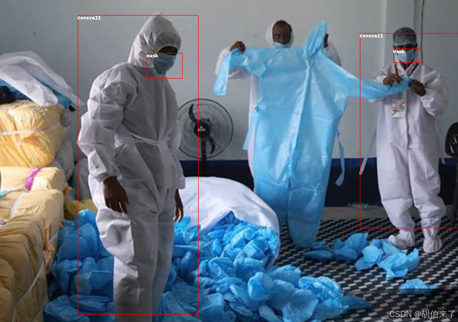
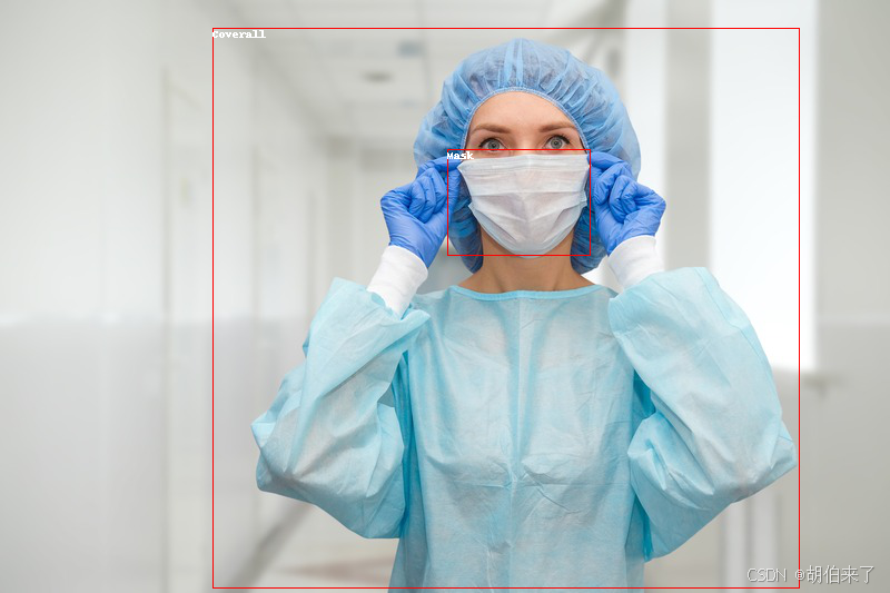
Detected Coverall with confidence 0.566 at location [1215.32, 147.38, 4401.81, 3227.08]
Detected Mask with confidence 0.584 at location [2449.06, 823.19, 3256.43, 1413.9]
现在我们来绘制结果吧:
draw = ImageDraw.Draw(image)

for score, label, box in zip(results["scores"], results["labels"], results["boxes"]):
     box = [round(i, 2) for i in box.tolist()]
     x, y, x2, y2 = tuple(box)
     draw.rectangle((x, y, x2, y2), outline="red", width=1)
     draw.text((x, y), model.config.id2label[label.item()], fill="white")

 image
结果:
零样本目标检测
传统上,用于目标检测的模型需要有标记的图像数据集进行训练,并且仅能检测训练集中的类别。
OWL-ViT 模型支持零样本目标检测,它使用了一种不同的方法。OWL-ViT 是一种开放词汇表的目标检测器,它可以根据自由文本查询在图像中检测对象,而无需在标记的数据集上对模型进行微调。
OWL-ViT 利用多模态表示来进行开放词汇表的检测。它将CLIP与轻量级的对象分类和定位头部结合起来。开放词汇表的检测是通过将自由文本查询与CLIP的文本编码器进行嵌入,并将其作为对象分类和定位头部的输入来实现的。 将图像及其相应的文本描述关联起来,ViT将图像块作为输入。OWL-ViT 的作者首先从头开始训练CLIP,然后使用二分匹配损失在标准目标检测数据集上端到端地对 OWL-ViT 进行微调。
采用这种方法,模型可以根据文本描述检测对象,而无需在标记的数据集上进行先前的训练。
开始之前,请确保你已安装所有必要的库:
pip install -q transformers零样本目标检测 pipeline
使用 OWL-ViT 进行推理的最简单方法是在`pipeline`中使用它:
from transformers import pipeline

checkpoint = "google/owlvit-base-patch32"
detector = pipeline(model=checkpoint, task="zero-shot-object-detection")
接下来,选择一张你想要检测对象的图片。这里我们将使用 NASA Great Images 数据集中的宇航员 Eileen Collins 的照片。
import skimage
import numpy as np
from PIL import Image

image = skimage.data.astronaut()
image = Image.fromarray(np.uint8(image)).convert("RGB")

image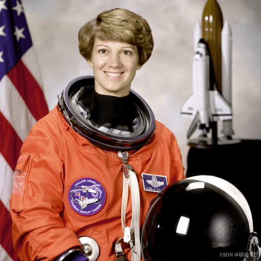
将图片和要查找的候选对象标签传递给 pipeline 。 这里我们直接传递了图片;其他合适的选项包括图像的本地路径或图像URL。我们还传递了要查询图像的所有物体的文本描述。
predictions = detector(
     image,
     candidate_labels=["human face", "rocket", "nasa badge", "star-spangled banner"],
 )
predictions
结果为:
[{'score': 0.3571370542049408,
  'label': 'human face',
  'box': {'xmin': 180, 'ymin': 71, 'xmax': 271, 'ymax': 178}},
 {'score': 0.28099656105041504,
  'label': 'nasa badge',
  'box': {'xmin': 129, 'ymin': 348, 'xmax': 206, 'ymax': 427}},
 {'score': 0.2110239565372467,
  'label': 'rocket',
  'box': {'xmin': 350, 'ymin': -1, 'xmax': 468, 'ymax': 288}},
 {'score': 0.13790413737297058,
  'label': 'star-spangled banner',
  'box': {'xmin': 1, 'ymin': 1, 'xmax': 105, 'ymax': 509}},
 {'score': 0.11950037628412247,
  'label': 'nasa badge',
  'box': {'xmin': 277, 'ymin': 338, 'xmax': 327, 'ymax': 380}},
 {'score': 0.10649408400058746,
  'label': 'rocket',
  'box': {'xmin': 358, 'ymin': 64, 'xmax': 424, 'ymax': 280}}]
让我们可视化预测结果:
from PIL import ImageDraw

draw = ImageDraw.Draw(image)

for prediction in predictions:
     box = prediction["box"]
     label = prediction["label"]
     score = prediction["score"]

     xmin, ymin, xmax, ymax = box.values()
     draw.rectangle((xmin, ymin, xmax, ymax), outline="red", width=1)
     draw.text((xmin, ymin), f"{label}: {round(score,2)}", fill="white")

image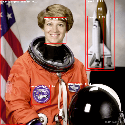
手动进行文本启发的零样本目标检测
现在,你已经了解了如何使用零样本目标检测的pipeline,让我们手动复制相同的结果。
首先从 Hub上的检查点 加载模型和相关的 processor。 这里我们将使用与之前相同的检查点:
from transformers import AutoProcessor, AutoModelForZeroShotObjectDetection

model = AutoModelForZeroShotObjectDetection.from_pretrained(checkpoint)
processor = AutoProcessor.from_pretrained(checkpoint)
我们选取不同的图片来稍微改变一下。
import requests

url = "https://unsplash.com/photos/oj0zeY2Ltk4/download?ixid=MnwxMjA3fDB8MXxzZWFyY2h8MTR8fHBpY25pY3xlbnwwfHx8fDE2Nzc0OTE1NDk&force=true&w=640"
im = Image.open(requests.get(url, stream=True).raw)
im
使用 processor 来准备模型的输入。processor 使用图像处理器对图像进行调整和归一化,以便模型处理,并且使用相应的`CLIPTokenizer`处理文本输入。
text_queries = ["hat", "book", "sunglasses", "camera"]
inputs = processor(text=text_queries, images=im, return_tensors="pt")将输入传递给模型,进行后处理和可视化结果。由于图像处理器在将图像馈送给模型之前会调整图像大小,因此你需要使用`~OwlViTImageProcessor.post_process_object_detection`方法来确保预测的边界框相对于原始图像具有正确的坐标:
import torch

with torch.no_grad():
     outputs = model(**inputs)
     target_sizes = torch.tensor([im.size[::-1]])
     results = processor.post_process_object_detection(outputs, threshold=0.1, target_sizes=target_sizes)[0]

draw = ImageDraw.Draw(im)

scores = results["scores"].tolist()
labels = results["labels"].tolist()
boxes = results["boxes"].tolist()

for box, score, label in zip(boxes, scores, labels):
     xmin, ymin, xmax, ymax = box
     draw.rectangle((xmin, ymin, xmax, ymax), outline="red", width=1)
     draw.text((xmin, ymin), f"{text_queries[label]}: {round(score,2)}", fill="white")

im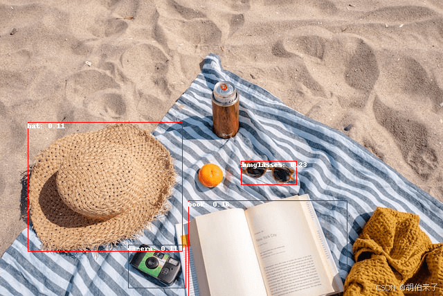
批量处理
你可以传递多组图像和文本查询来搜索一个或多个图像中的不同(或相同)对象。 让我们一起使用宇航员图像和海滩图像。 对于批量处理,你应该将文本查询作为处理器的嵌套列表传递,并将图像作为PIL图像,PyTorch 张量或 NumPy 数组的列表传递。
images = [image, im]
text_queries = [
     ["human face", "rocket", "nasa badge", "star-spangled banner"],
     ["hat", "book", "sunglasses", "camera"],
 ]
inputs = processor(text=text_queries, images=images, return_tensors="pt")之前后处理时使用了图片的大小的单个张量,但是也可以传递一个元组,或者在存在多张图像的情况下,传递一个元组列表。让我们为两个例子创建预测,并可视化第二个例子(image_idx = 1)。
with torch.no_grad():
     outputs = model(**inputs)
     target_sizes = [x.size[::-1] for x in images]
     results = processor.post_process_object_detection(outputs, threshold=0.1, target_sizes=target_sizes)

image_idx = 1
draw = ImageDraw.Draw(images[image_idx])

scores = results[image_idx]["scores"].tolist()
labels = results[image_idx]["labels"].tolist()
boxes = results[image_idx]["boxes"].tolist()

for box, score, label in zip(boxes, scores, labels):
     xmin, ymin, xmax, ymax = box
     draw.rectangle((xmin, ymin, xmax, ymax), outline="red", width=1)
     draw.text((xmin, ymin), f"{text_queries[image_idx][label]}: {round(score,2)}", fill="white")

images[image_idx]
图像引导的目标检测
除了使用文本查询进行零样本目标检测外,OWL-ViT 还提供了图像引导的目标检测。这意味着你可以使用图像查询在目标图像中查找相似的对象。 与文本查询不同,图像查询只允许一个示例图像。
让我们以一个有两只猫的沙发图像作为目标图像,并以单个猫的图像作为查询:
url = "http://images.cocodataset.org/val2017/000000039769.jpg"
image_target = Image.open(requests.get(url, stream=True).raw)

query_url = "http://images.cocodataset.org/val2017/000000524280.jpg"
query_image = Image.open(requests.get(query_url, stream=True).raw)
让我们快速查看一下这些图像:
import matplotlib.pyplot as plt

fig, ax = plt.subplots(1, 2)
ax[0].imshow(image_target)
ax[1].imshow(query_image)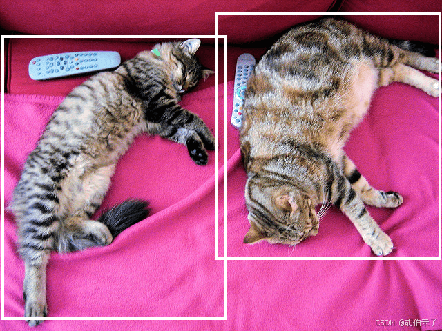
在预处理步骤中,不再使用文本查询,而是需要使用query_images:
inputs = processor(images=image_target, query_images=query_image, return_tensors="pt")对于预测,不再将输入传递给模型,而是将其传递给`~OwlViTForObjectDetection.image_guided_detection`。像以前一样绘制预测,只是现在没有标签了。
with torch.no_grad():
     outputs = model.image_guided_detection(**inputs)
     target_sizes = torch.tensor([image_target.size[::-1]])
     results = processor.post_process_image_guided_detection(outputs=outputs, target_sizes=target_sizes)[0]

draw = ImageDraw.Draw(image_target)

scores = results["scores"].tolist()
boxes = results["boxes"].tolist()

for box, score, label in zip(boxes, scores, labels):
     xmin, ymin, xmax, ymax = box
     draw.rectangle((xmin, ymin, xmax, ymax), outline="white", width=4)

image_target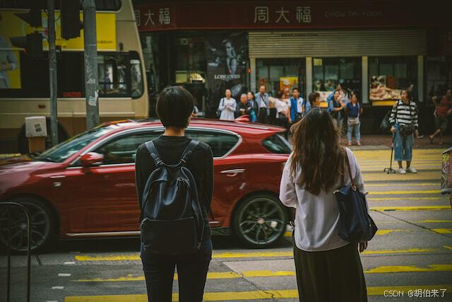
深度估计
单目深度估计是一项计算机视觉任务,涉及从单个图像中预测场景的深度信息。换句话说,它是从单个摄像机视角估计场景中对象的距离的过程。
单目深度估计具有各种应用,包括3D重建、增强现实、自动驾驶和机器人技术。这是一项具有挑战性的任务,因为它要求模型理解场景中对象之间的复杂关系和相应的深度信息,这些信息可能受到照明条件、遮挡和纹理等因素的影响。
该任务由以下模型架构支持:
DPT,GLPN
开始之前,请确保已安装所有必要的库:
pip install -q transformers深度估计流水线
尝试使用支持深度估计的模型进行推理的最简单方法是使用相应的 `pipeline` 实例化一个流水线。 可以从Hugging Face Hub上的检查点中实例化一个流水线:
from transformers import pipeline

checkpoint = "vinvino02/glpn-nyu"
depth_estimator = pipeline("depth-estimation", model=checkpoint)
接下来,选择一个要分析的图像:
from PIL import Image
import requests

url = "https://unsplash.com/photos/HwBAsSbPBDU/download?ixid=MnwxMjA3fDB8MXxzZWFyY2h8MzR8fGNhciUyMGluJTIwdGhlJTIwc3RyZWV0fGVufDB8MHx8fDE2Nzg5MDEwODg&force=true&w=640"
image = Image.open(requests.get(url, stream=True).raw)
image
将图像传递给流水线。
predictions = depth_estimator(image)流水线返回一个包含两个条目的字典。第一个条目称为 predicted_depth,是一个张量,其值表示每个像素的深度,以米为单位。 第二个条目 depth 是一个 PIL 图像,用于可视化深度估计结果。
让我们来看看可视化结果:
predictions["depth"]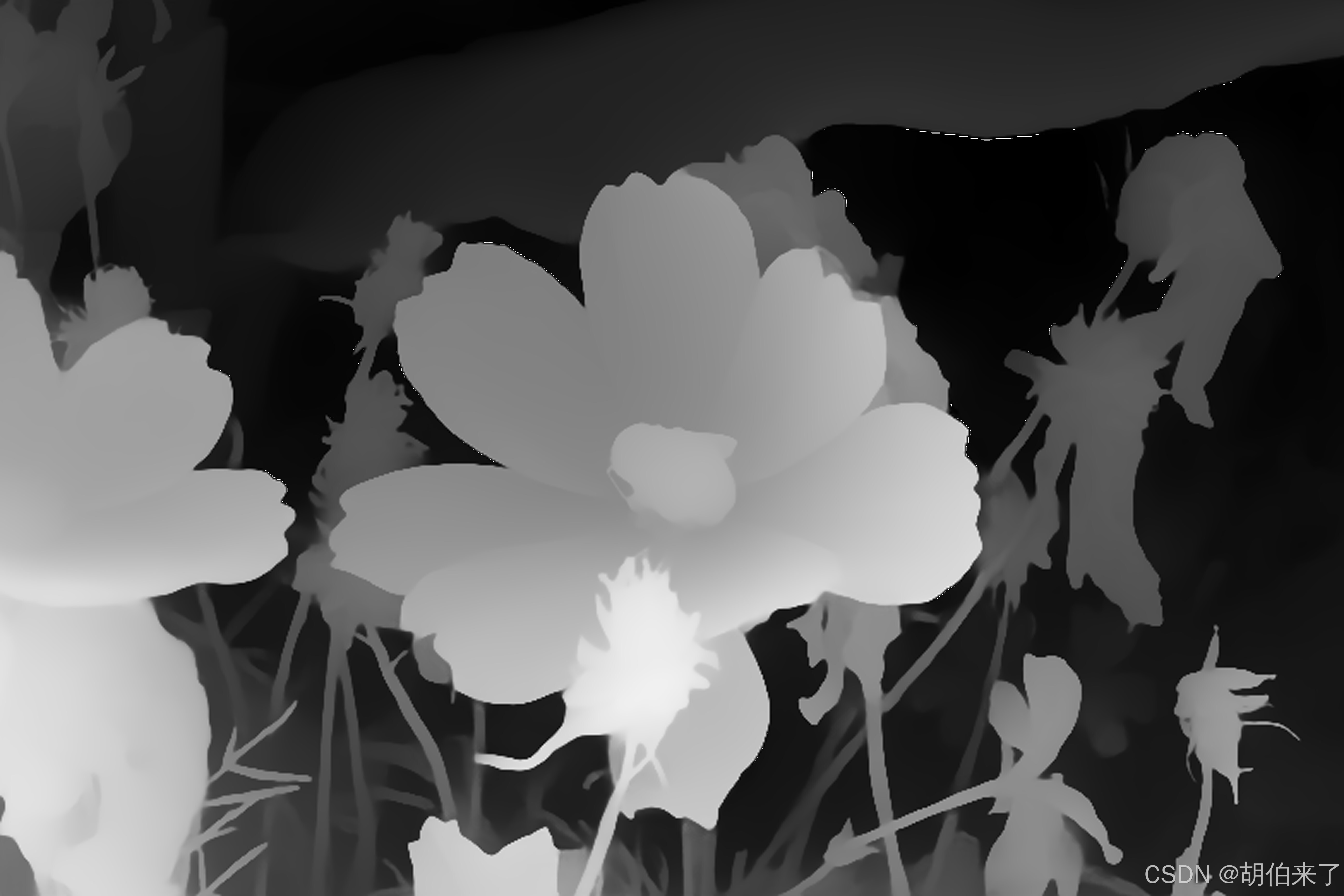
手动进行深度估计推理
现在,你已经了解如何使用深度估计流水线,让我们看看如何手动复制相同的结果。
从Hugging Face Hub上的检查点加载模型和相关处理器。 这里我们将使用之前相同的检查点:
from transformers import AutoImageProcessor, AutoModelForDepthEstimation

checkpoint = "vinvino02/glpn-nyu"

image_processor = AutoImageProcessor.from_pretrained(checkpoint)
model = AutoModelForDepthEstimation.from_pretrained(checkpoint)
使用 image_processor 准备图像输入,它将负责必要的图像变换,如调整大小和归一化:
pixel_values = image_processor(image, return_tensors="pt").pixel_values将准备好的输入传递给模型:
import torch

with torch.no_grad():
     outputs = model(pixel_values)
     predicted_depth = outputs.predicted_depth
可视化结果:
import numpy as np

# 插值到原始大小
prediction = torch.nn.functional.interpolate(
     predicted_depth.unsqueeze(1),
     size=image.size[::-1],
     mode="bicubic",
     align_corners=False,
 ).squeeze()
output = prediction.numpy()

formatted = (output * 255 / np.max(output)).astype("uint8")
depth = Image.fromarray(formatted)
depth
视频分类
视频分类(Video classification)是为整个视频分配标签或类别的任务,预期每个视频只能有一个分类。视频分类模型将视频作为输入,并预测视频属于哪个类。视频分类的一个实际应用是动作/活动识别,这对健身应用和视力受损的人都很有用。
本章节所示的任务支持TimeSformer, VideoMAE, ViViT等模型架构。
开始之前,请确保你已安装所有必要的库:
pip install -q pytorchvideo transformers evaluate你将使用 PyTorchVideo(也写为 PyTorchVideo)来处理和准备视频。
加载 UCF101 数据集
首先加载 UCF-101 数据集的一个子集。在对整个数据集进行更长时间的训练之前,通过在子集上进行实验并确保一切正常运行。
from huggingface_hub import hf_hub_download

hf_dataset_identifier = "sayakpaul/ucf101-subset"
filename = "UCF101_subset.tar.gz"
file_path = hf_hub_download(repo_id=hf_dataset_identifier, filename=filename, repo_type="dataset")
下载完子集后,你需要解压缩存档:
import tarfile

with tarfile.open(file_path) as t:
      t.extractall(".")
在更高层次的应用上,数据集的组织方式如下:
UCF101_subset/
    train/
        BandMarching/
            video_1.mp4
            video_2.mp4
            ...
        Archery
            video_1.mp4
            video_2.mp4
            ...
        ...
    val/
        BandMarching/
            video_1.mp4
            video_2.mp4
            ...
        Archery
            video_1.mp4
            video_2.mp4
            ...
        ...
    test/
        BandMarching/
            video_1.mp4
            video_2.mp4
            ...
        Archery
            video_1.mp4
            video_2.mp4
            ...
        ...
(排序)视频路径如下所示:
'UCF101_subset/train/ApplyEyeMakeup/v_ApplyEyeMakeup_g07_c04.avi',
'UCF101_subset/train/ApplyEyeMakeup/v_ApplyEyeMakeup_g07_c06.avi',
'UCF101_subset/train/ApplyEyeMakeup/v_ApplyEyeMakeup_g08_c01.avi',
'UCF101_subset/train/ApplyEyeMakeup/v_ApplyEyeMakeup_g09_c02.avi',
'UCF101_subset/train/ApplyEyeMakeup/v_ApplyEyeMakeup_g09_c06.avi'你将注意到,同一组/场景中的视频剪辑属于同一组,其中组在视频文件路径中以g表示。例如,v_ApplyEyeMakeup_g07_c04.avi 和 v_ApplyEyeMakeup_g07_c06.avi。
对于验证和评估集,你不希望具有来自同一组/场景的视频剪辑,以防止数据泄漏。
接下来,你将提取数据集中的标签集。同时,创建两个在初始化模型时会有帮助的字典:
-
label2id:将类名映射到整数。 -
id2label:将整数映射到类名。class_labels = sorted({str(path).split("/")[2] for path in all_video_file_paths})
label2id = {label: i for i, label in enumerate(class_labels)}
id2label = {i: label for label, i in label2id.items()}print(f"Unique classes: {list(label2id.keys())}.")
结果:
# Unique classes: ['ApplyEyeMakeup', 'ApplyLipstick', 'Archery', 'BabyCrawling', 'BalanceBeam', 'BandMarching', 'BaseballPitch', 'Basketball', 'BasketballDunk', 'BenchPress'].有10个唯一类别。对于每个类别,训练集有30个视频。
加载要微调的模型
从预训练检查点和其相关联的图像处理器实例化视频分类模型。模型的编码器带有预训练参数,并且分类头是随机初始化的。在编写数据集的预处理流水线时,图像处理器将非常有用。
from transformers import VideoMAEImageProcessor, VideoMAEForVideoClassification

model_ckpt = "MCG-NJU/videomae-base"
image_processor = VideoMAEImageProcessor.from_pretrained(model_ckpt)
model = VideoMAEForVideoClassification.from_pretrained(
     model_ckpt,
     label2id=label2id,
     id2label=id2label,
     ignore_mismatched_sizes=True,  # 此参数表示你打算对已经微调过的检查点进行微调
 )
在模型加载过程中,你可能会注意到如下警告:
Some weights of the model checkpoint at MCG-NJU/videomae-base were not used when initializing VideoMAEForVideoClassification: [..., 'decoder.decoder_layers.1.attention.output.dense.bias', 'decoder.decoder_layers.2.attention.attention.key.weight']
- This IS expected if you are initializing VideoMAEForVideoClassification from the checkpoint of a model trained on another task or with another architecture (e.g. initializing a BertForSequenceClassification model from a BertForPreTraining model).
- This IS NOT expected if you are initializing VideoMAEForVideoClassification from the checkpoint of a model that you expect to be exactly identical (initializing a BertForSequenceClassification model from a BertForSequenceClassification model).
Some weights of VideoMAEForVideoClassification were not initialized from the model checkpoint at MCG-NJU/videomae-base and are newly initialized: ['classifier.bias', 'classifier.weight']
You should probably TRAIN this model on a down-stream task to be able to use it for predictions and inference.
警告告诉我们,我们丢弃了一些权重(例如 classifier 层的权重和偏差),并且随机初始化了另一些权重(新的 classifier 层的权重和偏差)。这在这种情况下是正常的,因为我们添加了一个新的头部,我们没有预训练权重,因此库警告我们在使用它进行推断之前应先微调此模型,而这正是我们要做的。
注意,此检查点在此任务的性能上更好,因为此检查点通过微调获得,微调时与此任务的域有很大的重叠。你可以查看此检查点,该检查点通过微调了 MCG-NJU/videomae-base-finetuned-kinetics 检查点而获得。
准备训练数据集
要预处理视频,你将利用 PyTorchVideo 库。首先导入所需的依赖项。
import pytorchvideo.data

from pytorchvideo.transforms import (
     ApplyTransformToKey,
     Normalize,
     RandomShortSideScale,
     RemoveKey,
     ShortSideScale,
     UniformTemporalSubsample,
 )

from torchvision.transforms import (
     Compose,
     Lambda,
     RandomCrop,
     RandomHorizontalFlip,
     Resize,
 )
对于训练数据集,使用统一的时间子采样、像素归一化、随机裁剪和随机水平翻转的组合作为转换。对于验证和评估数据集,保持相同的变换链,除了随机裁剪和水平翻转。
使用与预训练模型关联的 image_processor 来获取以下信息:
图像均值和标准差,用于对视频帧像素进行归一化。
视频帧将被调整为的空间分辨率。
首先定义一些常量。
mean = image_processor.image_mean
std = image_processor.image_std
if "shortest_edge" in image_processor.size:
     height = width = image_processor.size["shortest_edge"]
else:
     height = image_processor.size["height"]
     width = image_processor.size["width"]
resize_to = (height, width)

num_frames_to_sample = model.config.num_frames
sample_rate = 4
fps = 30
clip_duration = num_frames_to_sample * sample_rate / fps
现在,定义数据集特定的转换和数据集。
首先是训练集:
train_transform = Compose(
     [
         ApplyTransformToKey(
             key="video",
             transform=Compose(
                 [
                     UniformTemporalSubsample(num_frames_to_sample),
                     Lambda(lambda x: x / 255.0),
                     Normalize(mean, std),
                     RandomShortSideScale(min_size=256, max_size=320),
                     RandomCrop(resize_to),
                     RandomHorizontalFlip(p=0.5),
                 ]
             ),
         ),
     ]
 )

train_dataset = pytorchvideo.data.Ucf101(
     data_path=os.path.join(dataset_root_path, "train"),
     clip_sampler=pytorchvideo.data.make_clip_sampler("random", clip_duration),
     decode_audio=False,
     transform=train_transform,
 )
相同的工作流程也适用于验证和评估集:
val_transform = Compose(
     [
         ApplyTransformToKey(
             key="video",
             transform=Compose(
                 [
                     UniformTemporalSubsample(num_frames_to_sample),
                     Lambda(lambda x: x / 255.0),
                     Normalize(mean, std),
                     Resize(resize_to),
                 ]
             ),
         ),
     ]
 )

val_dataset = pytorchvideo.data.Ucf101(
     data_path=os.path.join(dataset_root_path, "val"),
     clip_sampler=pytorchvideo.data.make_clip_sampler("uniform", clip_duration),
     decode_audio=False,
     transform=val_transform,
 )

test_dataset = pytorchvideo.data.Ucf101(
     data_path=os.path.join(dataset_root_path, "test"),
     clip_sampler=pytorchvideo.data.make_clip_sampler("uniform", clip_duration),
     decode_audio=False,
     transform=val_transform,
 )
注意:以上数据集流水线取自 PyTorchVideo 官方示例。我们使用 pytorchvideo.data.Ucf101() 函数,因为它专为 UCF-101 数据集定制。在幕后,它返回一个 pytorchvideo.data.labeled_video_dataset.LabeledVideoDataset 对象。 LabeledVideoDataset 类是 PyTorchVideo 数据集中与视频相关的基类。因此,如果要使用 PyTorchVideo 不支持的自定义数据集,可以相应地扩展 LabeledVideoDataset 类。
你可以访问 num_videos 参数以了解数据集中的视频数量。
print(train_dataset.num_videos, val_dataset.num_videos, test_dataset.num_videos)结果:
(300, 30, 75)可视化预处理的视频
import imageio
import numpy as np
from IPython.display import Image

def unnormalize_img(img):
     """Un-normalizes the image pixels."""
     img = (img * std) + mean
     img = (img * 255).astype("uint8")
     return img.clip(0, 255)

def create_gif(video_tensor, filename="sample.gif"):
     """Prepares a GIF from a video tensor.

     The video tensor is expected to have the following shape:
     (num_frames, num_channels, height, width).
     """
     frames = []
     for video_frame in video_tensor:
         frame_unnormalized = unnormalize_img(video_frame.permute(1, 2, 0).numpy())
         frames.append(frame_unnormalized)
     kargs = {"duration": 0.25}
     imageio.mimsave(filename, frames, "GIF", **kargs)
     return filename

def display_gif(video_tensor, gif_name="sample.gif"):
     """Prepares and displays a GIF from a video tensor."""
     video_tensor = video_tensor.permute(1, 0, 2, 3)
     gif_filename = create_gif(video_tensor, gif_name)
     return Image(filename=gif_filename)

sample_video = next(iter(train_dataset))
video_tensor = sample_video["video"]
display_gif(video_tensor)
训练模型
使用 Transformers 中的 Trainer 对模型进行训练。要实例化一个 Trainer,需要定义训练配置和评估指标。其中最重要的是 TrainingArguments,它是一个包含所有属性以配置训练的类。它需要一个输出文件夹名称,用于保存模型的检查点。它还有助于同步 Hub 上模型存储库中的所有信息。
大多数训练参数都是显而易见的,但这里有一个非常重要的参数 remove_unused_columns=False。它会丢弃模型的调用函数未使用的任何特征。默认情况下它是 True,因为通常丢弃未使用的特征列是理想的,这样可以更容易地将输入解包到模型的调用函数中。但是,在这种情况下,你需要未使用的特征(特别是 video)来创建 pixel_values(这是我们的模型在其输入中期望的一个必需键)。
下面代码定义了训练的参数:
from transformers import TrainingArguments, Trainer

model_name = model_ckpt.split("/")[-1]
new_model_name = f"{model_name}-finetuned-ucf101-subset"
num_epochs = 4

args = TrainingArguments(
     new_model_name,
     remove_unused_columns=False,
     evaluation_strategy="epoch",
     save_strategy="epoch",
     learning_rate=5e-5,
     per_device_train_batch_size=batch_size,
     per_device_eval_batch_size=batch_size,
     warmup_ratio=0.1,
     logging_steps=10,
     load_best_model_at_end=True,
     metric_for_best_model="accuracy",
     push_to_hub=True,
     max_steps=(train_dataset.num_videos // batch_size) * num_epochs,
 )
pytorchvideo.data.Ucf101() 返回的数据集没有实现 __len__ 方法。因此,在实例化 TrainingArguments 时,我们必须定义 max_steps。
下一步,你需要定义一个用于根据预测结果计算度量标准的函数,该函数将使用你将要加载的 metric。你唯一需要做的预处理就是获取预测 logits 的 argmax:
import evaluate

metric = evaluate.load("accuracy")

def compute_metrics(eval_pred):
    predictions = np.argmax(eval_pred.predictions, axis=1)
    return metric.compute(predictions=predictions, references=eval_pred.label_ids)
💡 关于评估的说明
在
VideoMAE论文 中,作者使用以下评估策略。他们对测试视频中的几个片段进行评估,并对这些片段应用不同的裁剪,并报告聚合分数。然而,在简洁和简洁的兴趣下,该教程中没有考虑这一点。还要定义一个
collate_fn,它将用于将示例批处理在一起。每个批处理包含pixel_values和labels这两个键。
def collate_fn(examples):
# permute to (num_frames, num_channels, height, width)
pixel_values = torch.stack(
[example["video"].permute(1, 0, 2, 3) for example in examples]
)
labels = torch.tensor([example["label"] for example in examples])
return {"pixel_values": pixel_values, "labels": labels}
然后,将所有这些和数据集一起传递给
Trainer:
trainer = Trainer(
model,
args,
train_dataset=train_dataset,
eval_dataset=val_dataset,
tokenizer=image_processor,
compute_metrics=compute_metrics,
data_collator=collate_fn,
)
你可能想知道为什么在预处理数据时已经将
image_processor作为tokenizer传递了。这只是为了确保图像处理器配置文件(存储为JSON)也会上传到 Hub 上的仓库中。现在通过调用
train方法来微调我们的模型:
train_results = trainer.train()训练完成后,使用 `transformers.Trainer.push_to_hub` 方法将你的模型共享到 Hub 中,这样每个人都可以使用你的模型:
trainer.push_to_hub()
推理
现在你已经对模型进行了微调,可以用它进行推理了!
加载一个用于推理的视频:
sample_test_video = next(iter(test_dataset))在推理中尝试使用微调后的模型最简单的方法是在 pipeline 中使用它。使用你的模型实例化一个视频分类的 pipeline,并将视频传递给它:
from transformers import pipeline

video_cls = pipeline(model="my_awesome_video_cls_model")
video_cls("https://huggingface.co/datasets/sayakpaul/ucf101-subset/resolve/main/v_BasketballDunk_g14_c06.avi")
结果为:
[{'score': 0.9272987842559814, 'label': 'BasketballDunk'},
 {'score': 0.017777055501937866, 'label': 'BabyCrawling'},
 {'score': 0.01663011871278286, 'label': 'BalanceBeam'},
 {'score': 0.009560945443809032, 'label': 'BandMarching'},
 {'score': 0.0068979403004050255, 'label': 'BaseballPitch'}]
你也可以手动复制 pipeline 的结果。
def run_inference(model, video):
     # (num_frames, num_channels, height, width)
     perumuted_sample_test_video = video.permute(1, 0, 2, 3)
     inputs = {
         "pixel_values": perumuted_sample_test_video.unsqueeze(0),
         "labels": torch.tensor(
             [sample_test_video["label"]]
         ),  # 如果没有标签可用,可以跳过此项。
     }

     device = torch.device("cuda" if torch.cuda.is_available() else "cpu")
     inputs = {k: v.to(device) for k, v in inputs.items()}
     model = model.to(device)

     # 前向传递
     with torch.no_grad():
         outputs = model(**inputs)
         logits = outputs.logits

     return logits
现在,将输入传递给模型并返回 logits:
logits = run_inference(trained_model, sample_test_video["video"])解码 logits,我们得到:
predicted_class_idx = logits.argmax(-1).item()
print("Predicted class:", model.config.id2label[predicted_class_idx])
# Predicted class: BasketballDunk