自然语言处理实战——基于 BP 神经网络的中文文本情感分类

核心目标	区分中文文本的「正面情感」（如好评、开心）和「负面情感」（如差评、生气）
技术栈	纯 Numpy 实现 BP 神经网络 + TF-IDF 文本特征提取 + 中文分词（jieba） + 多维度可视化
数据流转	原始文本文件 → 文本预处理（分词 / 去停用词） → TF-IDF 数值特征 → BP 网络训练 → 模型评估 → 可视化分析 → 新样本预测

三、模块 1：环境配置与基础库导入

python 复制代码

import numpy as np
import jieba
import os
import warnings
warnings.filterwarnings('ignore')

# 可视化库
import matplotlib.pyplot as plt
import seaborn as sns
from wordcloud import WordCloud
from sklearn.metrics import confusion_matrix, classification_report, accuracy_score
from sklearn.feature_extraction.text import TfidfVectorizer
from sklearn.model_selection import train_test_split

# 设置中文字体（解决可视化中文乱码）
plt.rcParams['font.sans-serif'] = ['SimHei']  # 黑体
plt.rcParams['axes.unicode_minus'] = False  # 解决负号显示问题

功能说明：

基础库导入 ：
- numpy：手动实现 BP 神经网络的核心（矩阵运算、梯度计算）；
- jieba：中文文本分词（解决中文无天然分隔符的问题）；
- os：读取文本文件（路径处理）；
- warnings：屏蔽无关警告（提升运行体验）。
可视化库导入 ：
- matplotlib/seaborn：绘制损失曲线、混淆矩阵、特征重要性等图表；
- WordCloud：生成情感文本词云（直观展示核心词汇）。
SKlearn 工具导入 ：
- 特征提取：TfidfVectorizer（将文本转为数值特征）；
- 数据划分：train_test_split（拆分训练 / 测试集）；
- 模型评估：confusion_matrix/classification_report/accuracy_score（量化模型性能）。
中文显示配置：解决 Matplotlib 可视化时中文乱码、负号显示异常的问题。

四、模块 2：核心工具函数（数据处理 + 激活函数）

2.1 激活函数（神经网络核心）

python 复制代码

def sigmoid(z):
    """Sigmoid激活函数（数值稳定版）"""
    z = np.clip(z, -500, 500)  # 防止exp(-z)溢出（z过大/过小导致计算错误）
    return 1 / (1 + np.exp(-z))

def sigmoid_derivative(z):
    """Sigmoid导数（反向传播需计算激活函数梯度）"""
    s = sigmoid(z)
    return s * (1 - s)

def relu(z):
    """ReLU激活函数（隐藏层用，缓解梯度消失）"""
    return np.maximum(0, z)

def relu_derivative(z):
    """ReLU导数（反向传播用）"""
    return np.where(z > 0, 1, 0)

函数	作用	应用场景
`sigmoid`	将输出映射到 (0,1) 区间，适配二分类任务（情感分类的输出层）	输出层激活（判断 0/1 情感）
`sigmoid_derivative`	计算 Sigmoid 的导数，用于反向传播的梯度计算	输出层误差项推导
`relu`	隐藏层激活函数，计算快、缓解梯度消失（相比 Sigmoid 更适合深层网络）	隐藏层激活
`relu_derivative`	计算 ReLU 的导数，用于反向传播的梯度计算	隐藏层误差项推导

2.2 数据读取函数

python 复制代码

def load_sentiment_data(data_dir):
    """读取情感分类文本数据（从txt文件读取）"""
    texts = []
    labels = []

    # 读取正面文本（标签1）
    pos_path = os.path.join(data_dir, 'positive.txt')
    with open(pos_path, 'r', encoding='utf-8') as f:
        for line in f:
            line = line.strip()
            if line:  # 跳过空行
                texts.append(line)
                labels.append(1)

    # 读取负面文本（标签0）
    neg_path = os.path.join(data_dir, 'negative.txt')
    with open(neg_path, 'r', encoding='utf-8') as f:
        for line in f:
            line = line.strip()
            if line:  # 跳过空行
                texts.append(line)
                labels.append(0)

    return texts, np.array(labels).reshape(-1, 1)

功能说明：

输入：数据文件夹路径（sentiment_data）；
输出：文本列表（texts）、标签数组（labels，1 = 正面，0 = 负面，形状为(n_samples, 1)）；

核心逻辑：

读取positive.txt（正面文本），每行一条，标签设为 1；

bash 复制代码

这家餐厅的菜品超好吃，服务也特别周到
今天收到了心仪的礼物，心情超级棒
这部电影剧情紧凑，演员演技在线，值得一看
新入手的手机续航超久，拍照效果也很好
周末和朋友去郊游，天气好风景美，太开心了
公司团建活动很有趣，同事们都玩得很尽兴
这家咖啡店的拿铁口感丝滑，环境也很温馨
网购的衣服尺码很准，面料也很舒服
终于通过了考试，付出的努力都值得了
家乡的变化真大，基础设施越来越完善了

读取negative.txt（负面文本），每行一条，标签设为 0；

bash 复制代码

这家外卖送得超级慢，饭菜都凉了
手机用了没几天就卡顿，体验太差了
餐厅的菜品又贵又难吃，性价比极低
今天上班迟到被批评，一整天心情都不好
电影剧情拖沓，特效粗糙，完全不值票价
网购的商品有瑕疵，客服还不处理，太气人了
下雨天出门没带伞，被淋成落汤鸡了
公交车晚点半小时，耽误了重要的约会
这家酒店卫生条件差，房间还有异味
快递员态度恶劣，包裹还破损了

跳过空行，避免无效数据；
标签转为 Numpy 数组并重塑为列向量（适配 BP 网络的矩阵运算）。

2.3 文本预处理函数

python 复制代码

def preprocess_text(texts):
    """中文文本预处理：分词+去停用词"""
    # 简单停用词表（无实际语义，需过滤）
    stopwords = {'的', '了', '在', '是', '我', '你', '他', '她', '它', '们', '就', '都', '也', '还', '很', '太', '超',
                 '又', '和', '与', '及', '等', '有', '没', '不', '无', '为', '之', '于', '以', '对', '对于'}

    processed_texts = []
    for text in texts:
        # 分词（jieba.lcut：精确分词，返回列表）
        words = jieba.lcut(text)
        # 去停用词+去空字符（保留有语义的词汇）
        words = [w for w in words if w.strip() and w not in stopwords]
        processed_texts.append(' '.join(words))

    return processed_texts

功能说明：

输入：原始文本列表（如["这家餐厅超好吃", ...]）；
输出：预处理后的文本列表（如["这家餐厅好吃", ...]）；
核心价值：
1. 分词：将连续中文拆分为独立词汇（如 "超好吃"→"超好吃"），适配 TF-IDF 特征提取；
2. 去停用词：过滤无语义的虚词（如 "的""了"），减少噪声，提升特征有效性；
3. 格式转换：用空格分隔分词结果（TF-IDF 要求输入为 "词汇词汇" 格式）。

五、模块 3：BP 神经网络类（核心模型）

python 复制代码

class BPNeuralNetwork:
    def __init__(self, input_dim, hidden_dim, output_dim, learning_rate=0.01):
        # 初始化网络参数
        self.input_dim = input_dim  # 输入维度（TF-IDF特征数）
        self.hidden_dim = hidden_dim  # 隐藏层神经元数
        self.output_dim = output_dim  # 输出维度（二分类=1）
        self.lr = learning_rate  # 学习率（控制参数更新步长）

        # 权重初始化（Xavier初始化：适配ReLU，避免梯度消失/爆炸）
        self.W1 = np.random.normal(0, np.sqrt(2 / input_dim), (hidden_dim, input_dim))
        self.b1 = np.zeros((hidden_dim, 1))  # 隐藏层偏置（初始化为0）
        self.W2 = np.random.normal(0, np.sqrt(2 / hidden_dim), (output_dim, hidden_dim))
        self.b2 = np.zeros((output_dim, 1))  # 输出层偏置（初始化为0）

        # 记录训练损失（用于可视化损失曲线）
        self.train_loss_history = []

3.1 初始化方法（`init`）

核心参数：
- input_dim：输入层维度（如 TF-IDF 的 100 维特征）；
- hidden_dim：隐藏层神经元数（如 64，控制模型复杂度）；
- output_dim：输出层维度（二分类 = 1）；
- learning_rate：学习率（默认 0.01，控制参数更新速度）；
关键逻辑：
1. 权重初始化：采用 Xavier 初始化（针对 ReLU 优化），避免全 0 初始化（导致神经元输出相同）；
2. 偏置初始化：初始化为 0（不影响梯度计算，训练中自动调整）；
3. 损失记录：初始化空列表，保存每轮训练的损失值（用于可视化）。

3.2 前向传播（`forward`）

python 复制代码

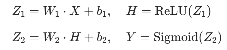
def forward(self, X):
    """前向传播：输入→隐藏层→输出层，计算预测值"""
    Z1 = np.dot(self.W1, X) + self.b1  # 隐藏层净输入（线性变换）
    H = relu(Z1)  # 隐藏层输出（ReLU激活）
    Z2 = np.dot(self.W2, H) + self.b2  # 输出层净输入（线性变换）
    Y = sigmoid(Z2)  # 输出层预测值（Sigmoid激活，范围0~1）
    return H, Y

输入：单个样本的特征向量（形状(input_dim, 1)）；
输出：隐藏层输出（H）、输出层预测值（Y，0~1 之间）；
核心逻辑：模拟信号在神经网络中的正向传递，公式对应：

3.3 反向传播（`backward`）

python 复制代码

def backward(self, X, H, Y, Y_true):
    """反向传播：计算损失对权重/偏置的梯度"""
    delta2 = Y - Y_true  # 输出层误差项（二元交叉熵+Sigmoid简化版）
    Z1 = np.dot(self.W1, X) + self.b1  # 重新计算隐藏层净输入
    delta1 = np.dot(self.W2.T, delta2) * relu_derivative(Z1)  # 隐藏层误差项

    # 计算各参数的梯度
    dW2 = np.dot(delta2, H.T)  # W2的梯度
    db2 = delta2  # b2的梯度
    dW1 = np.dot(delta1, X.T)  # W1的梯度
    db1 = delta1  # b1的梯度

    return dW1, db1, dW2, db2

输入：输入向量X、隐藏层输出H、预测值Y、真实标签Y_true；
输出：权重 / 偏置的梯度（dW1, db1, dW2, db2）；
核心逻辑（链式法则）：
1. 输出层误差项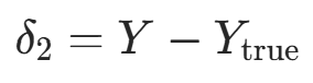：（二元交叉熵 + Sigmoid 的简化结果，无需复杂计算）；
2. 隐藏层误差项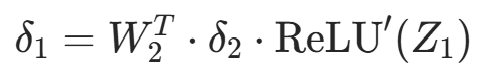：（通过输出层误差反向推导）；
3. 梯度计算：损失对每个参数的偏导数（用于后续参数更新）。

3.4 参数更新（`update_params`）

python 复制代码

def update_params(self, dW1, db1, dW2, db2):
    """梯度下降更新权重/偏置（沿梯度负方向调整，减小损失）"""
    self.W1 -= self.lr * dW1
    self.b1 -= self.lr * db1
    self.W2 -= self.lr * dW2
    self.b2 -= self.lr * db2

核心公式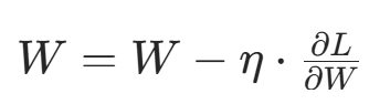：（η= 学习率，梯度负方向）；
作用：通过梯度下降最小化损失，让模型逐渐拟合数据规律。

3.5 训练函数（`train`）

python 复制代码

def train(self, X_train, y_train, epochs=50, batch_size=4):
    """迭代训练网络，记录每轮损失"""
    n_samples = X_train.shape[0]
    self.train_loss_history = []  # 重置损失记录

    for epoch in range(epochs):
        # 打乱训练集（避免顺序影响，提升泛化）
        indices = np.random.permutation(n_samples)
        X_shuffled = X_train[indices]
        y_shuffled = y_train[indices]

        epoch_loss = 0.0
        batch_count = 0

        # 批量训练（按batch_size切分）
        for i in range(0, n_samples, batch_size):
            batch_X = X_shuffled[i:i + batch_size]
            batch_y = y_shuffled[i:i + batch_size]
            batch_count += 1

            batch_batch_loss = 0.0
            for X, y_true in zip(batch_X, batch_y):
                # 重塑为列向量（适配矩阵运算）
                X = X.reshape(self.input_dim, 1)
                y_true = y_true.reshape(self.output_dim, 1)

                # 前向传播
                H, Y = self.forward(X)
                # 计算损失（加1e-7避免log(0)）
                loss = -y_true * np.log(Y + 1e-7) - (1 - y_true) * np.log(1 - Y + 1e-7)
                batch_batch_loss += loss.item()

                # 反向传播+参数更新
                dW1, db1, dW2, db2 = self.backward(X, H, Y, y_true)
                self.update_params(dW1, db1, dW2, db2)

            # 累加批量损失
            epoch_loss += batch_batch_loss / len(batch_X)

        # 记录每轮平均损失
        avg_epoch_loss = epoch_loss / batch_count
        self.train_loss_history.append(avg_epoch_loss)

        # 每5轮打印损失（监控训练进度）
        if (epoch + 1) % 5 == 0:
            print(f"Epoch {epoch + 1}/{epochs}, Average Loss: {avg_epoch_loss:.4f}")

核心参数：
- epochs：训练轮数（默认 50，遍历训练集的次数）；
- batch_size：批量大小（默认 4，小批量训练提升泛化）；
核心逻辑：
1. 每轮训练前打乱数据（避免顺序偏差）；
2. 按batch_size切分训练集，逐批处理；
3. 对每个样本：重塑为列向量→前向传播→计算损失→反向传播→更新参数；
4. 计算每轮平均损失并记录（用于可视化）；
5. 每 5 轮打印损失（方便监控训练收敛情况）；
6. 损失计算时加1e-7（避免log(0)导致数值错误）。

3.6 预测函数（`predict`）

python 复制代码

def predict(self, X):
    """预测函数：输入特征→输出情感标签（0/1）"""
    predictions = []
    for x in X:
        x = x.reshape(self.input_dim, 1)  # 重塑为列向量
        _, Y = self.forward(x)  # 前向传播获取预测值
        pred = 1 if Y > 0.5 else 0  # 阈值0.5：>0.5=正面，否则=负面
        predictions.append(pred)
    return np.array(predictions)

输入：测试集 / 新样本的特征矩阵（n_samples, input_dim）；
输出：预测标签数组（0 = 负面，1 = 正面）；
核心逻辑：
1. 对每个样本前向传播，得到 0~1 的预测值；
2. 以 0.5 为阈值，将连续值转为离散标签（二分类）。

六、模块 4：可视化函数（模型分析核心）

4.1 训练损失曲线（`plot_train_loss`）

python 复制代码

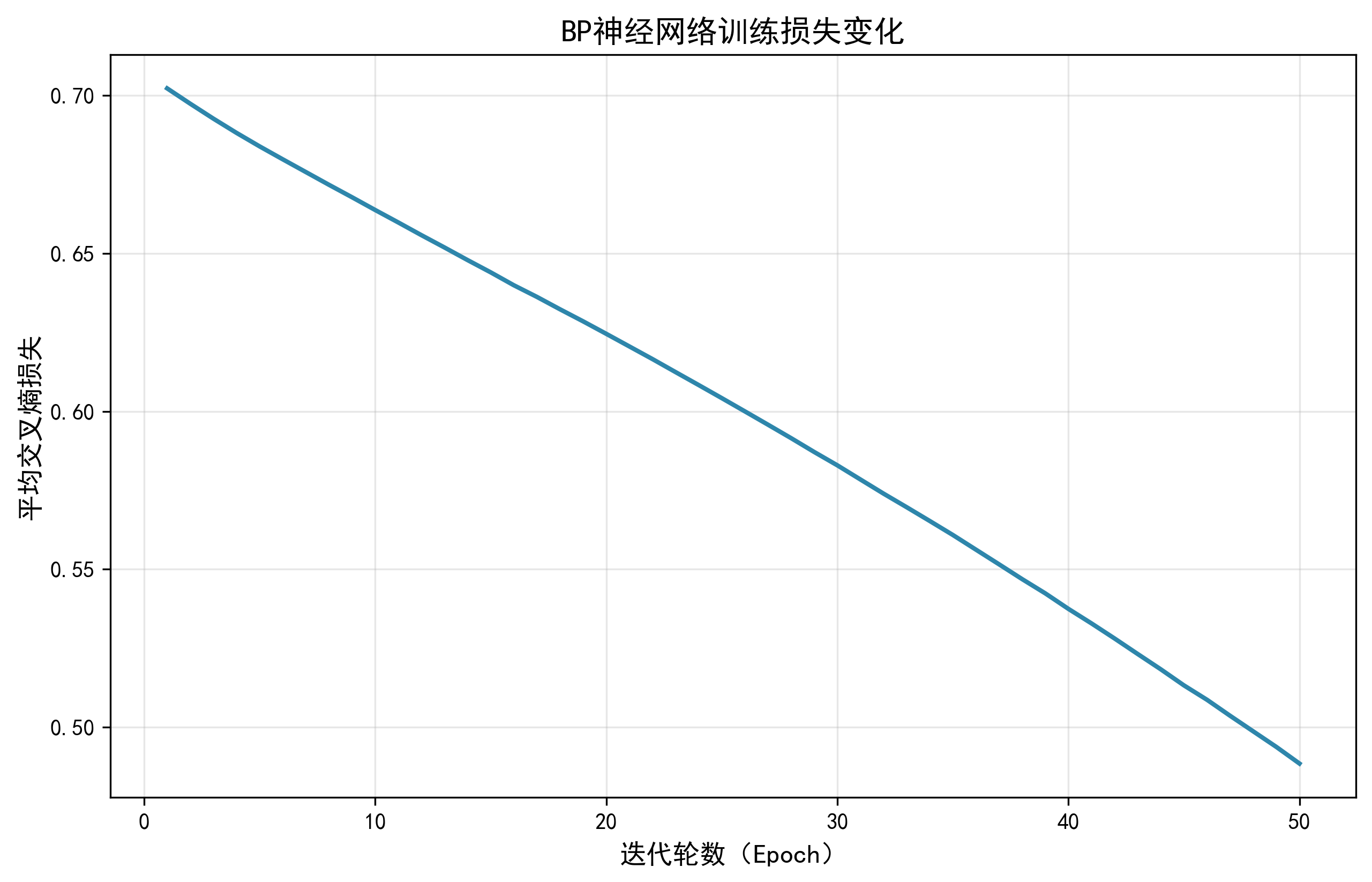
def plot_train_loss(loss_history):
    """绘制训练损失曲线（监控模型收敛）"""
    plt.figure(figsize=(10, 6))
    plt.plot(range(1, len(loss_history) + 1), loss_history, color='#2E86AB', linewidth=2)
    plt.title('BP神经网络训练损失变化', fontsize=14)
    plt.xlabel('迭代轮数（Epoch）', fontsize=12)
    plt.ylabel('平均交叉熵损失', fontsize=12)
    plt.grid(alpha=0.3)
    plt.savefig('train_loss_curve.png', dpi=300, bbox_inches='tight')
    plt.show()

功能：绘制 "迭代轮数→损失值" 曲线；
核心价值：
1. 查看损失是否下降并收敛（损失逐渐降低→模型学习有效）；
2. 判断过拟合 / 欠拟合（损失骤降后反弹→过拟合；损失不降→欠拟合）；
3. 保存高清图片（dpi=300），便于分析。

4.2 混淆矩阵热力图（`plot_confusion_matrix`）

python 复制代码

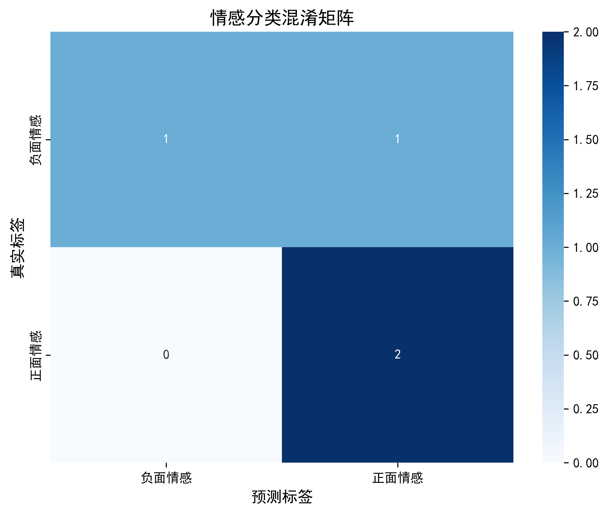
def plot_confusion_matrix(y_true, y_pred):
    """绘制混淆矩阵（查看分类错误类型）"""
    cm = confusion_matrix(y_true, y_pred)
    plt.figure(figsize=(8, 6))
    sns.heatmap(cm, annot=True, fmt='d', cmap='Blues',
                xticklabels=['负面情感', '正面情感'],
                yticklabels=['负面情感', '正面情感'])
    plt.title('情感分类混淆矩阵', fontsize=14)
    plt.xlabel('预测标签', fontsize=12)
    plt.ylabel('真实标签', fontsize=12)
    plt.savefig('confusion_matrix.png', dpi=300, bbox_inches='tight')
    plt.show()

功能：可视化混淆矩阵（行 = 真实标签，列 = 预测标签）；
核心价值：
1. 直观查看 "真阳性（正面预测正确）、真阴性（负面预测正确）、假阳性（负面误判为正面）、假阴性（正面误判为负面）"；
2. 定位模型薄弱点（如假阴性多→模型漏判正面情感）。

4.3 分类性能指标可视化（`plot_classification_report`）

python 复制代码

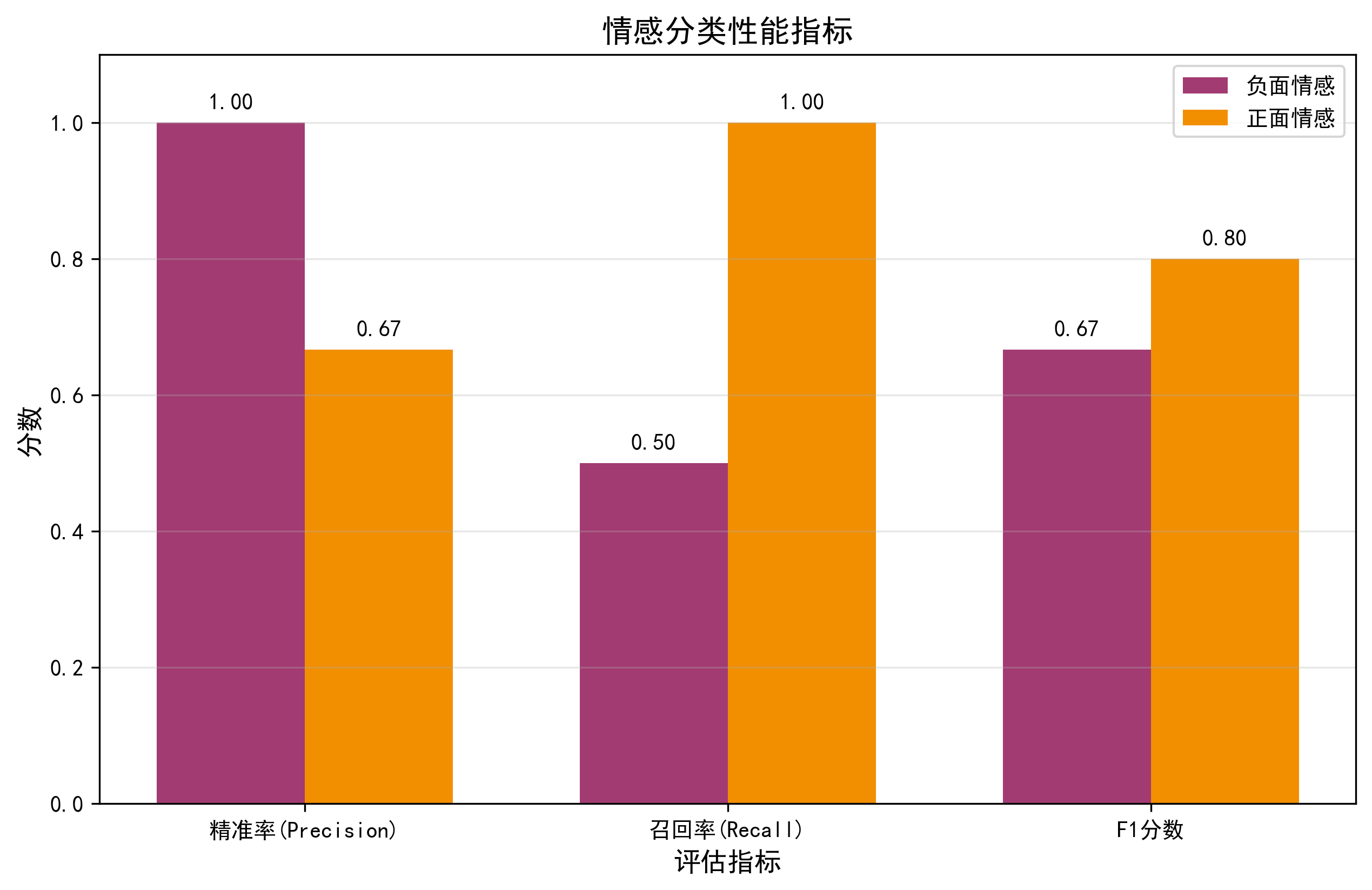
def plot_classification_report(y_true, y_pred):
    """可视化精准率、召回率、F1分数（量化模型性能）"""
    report = classification_report(y_true, y_pred, target_names=['负面情感', '正面情感'], output_dict=True)
    metrics = ['precision', 'recall', 'f1-score']
    pos_scores = [report['正面情感'][m] for m in metrics]
    neg_scores = [report['负面情感'][m] for m in metrics]

    x = np.arange(len(metrics))
    width = 0.35

    plt.figure(figsize=(10, 6))
    plt.bar(x - width / 2, neg_scores, width, label='负面情感', color='#A23B72')
    plt.bar(x + width / 2, pos_scores, width, label='正面情感', color='#F18F01')

    plt.title('情感分类性能指标', fontsize=14)
    plt.xlabel('评估指标', fontsize=12)
    plt.ylabel('分数', fontsize=12)
    plt.xticks(x, ['精准率(Precision)', '召回率(Recall)', 'F1分数'])
    plt.ylim(0, 1.1)
    plt.legend()

    # 添加数值标签（直观查看分数）
    for i, v in enumerate(neg_scores):
        plt.text(i - width / 2, v + 0.02, f'{v:.2f}', ha='center')
    for i, v in enumerate(pos_scores):
        plt.text(i + width / 2, v + 0.02, f'{v:.2f}', ha='center')

    plt.grid(alpha=0.3, axis='y')
    plt.savefig('classification_report.png', dpi=300, bbox_inches='tight')
    plt.show()

核心指标解释：
- 精准率（Precision）：预测为某类的样本中，真实为该类的比例（如正面精准率 = 正面预测正确 / 所有预测为正面）；
- 召回率（Recall）：真实为某类的样本中，预测正确的比例（如正面召回率 = 正面预测正确 / 所有真实正面）；
- F1 分数：精准率 + 召回率的调和平均（综合评估，越接近 1 越好）；
核心价值：量化对比正负情感的分类效果（如正面 F1=0.95，负面 F1=0.90→模型对正面分类更准）。

4.4 情感词云（`generate_wordcloud`）

python 复制代码

def generate_wordcloud(texts, label, save_path):
    """生成正负情感文本词云（直观展示核心词汇）"""
    text = ' '.join(texts)
    wc = WordCloud(
        font_path='simhei.ttf',  # 中文分词字体（需系统有该字体）
        width=800, height=600,
        background_color='white',
        max_words=100,
        colormap='RdYlGn' if label == 1 else 'RdYlBu_r'  # 正面=绿红，负面=蓝红
    ).generate(text)

    plt.figure(figsize=(10, 8))
    plt.imshow(wc, interpolation='bilinear')
    plt.axis('off')
    plt.title(f'{"正面" if label == 1 else "负面"}情感文本词云', fontsize=14)
    plt.savefig(save_path, dpi=300, bbox_inches='tight')
    plt.show()

功能：生成正负情感文本的词云（词汇越大→出现频率越高）；
核心价值：
1. 直观展示情感文本的核心词汇（如正面 ="好吃、开心、棒"；负面 ="慢、差、气"）；
2. 验证预处理效果（停用词是否过滤干净）；
3. 辅助业务分析（如负面词云多为 "慢"→优化配送效率）。

4.5 特征重要性（`plot_feature_importance`）

python 复制代码

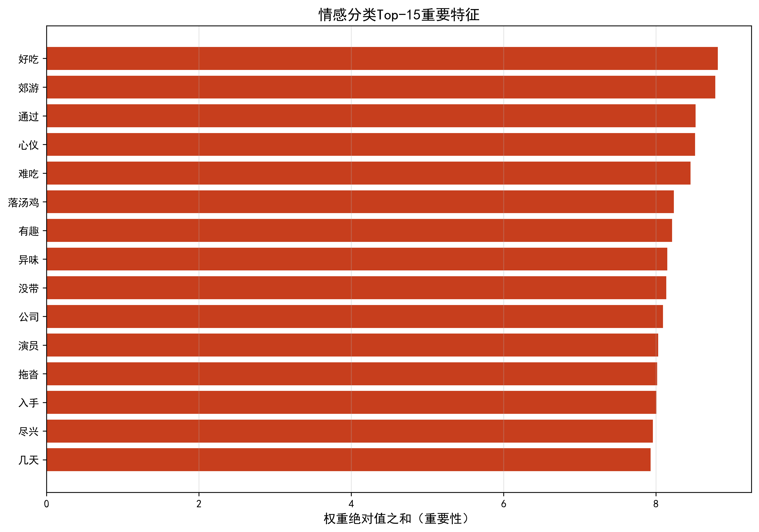
def plot_feature_importance(tfidf, model, top_k=15):
    """绘制Top-K重要特征（基于BP网络第一层权重）"""
    # 计算每个特征的权重绝对值之和（代表重要性）
    feature_importance = np.sum(np.abs(model.W1), axis=0)
    feature_names = tfidf.get_feature_names_out()  # 获取特征对应的词汇

    # 排序取Top-K
    indices = np.argsort(feature_importance)[-top_k:]
    top_importance = feature_importance[indices]
    top_features = feature_names[indices]

    # 绘制水平条形图
    plt.figure(figsize=(12, 8))
    plt.barh(range(len(top_features)), top_importance, color='#C73E1D')
    plt.yticks(range(len(top_features)), top_features)
    plt.title(f'情感分类Top-{top_k}重要特征', fontsize=14)
    plt.xlabel('权重绝对值之和（重要性）', fontsize=12)
    plt.grid(alpha=0.3, axis='x')
    plt.savefig('feature_importance.png', dpi=300, bbox_inches='tight')
    plt.show()

核心逻辑：BP 网络第一层权重的绝对值之和越大→该特征（词汇）对情感分类的影响越大；
核心价值：
1. 找出对情感分类最关键的词汇（如 "好吃""难吃""开心""生气"）；
2. 验证特征提取的有效性（关键词汇是否被选中）。

七、模块 5：主流程（整合所有功能）

python 复制代码

if __name__ == "__main__":
    # 1. 配置参数
    DATA_DIR = 'sentiment_data'  # 数据文件夹
    HIDDEN_DIM = 64  # 隐藏层神经元数
    LEARNING_RATE = 0.01  # 学习率
    EPOCHS = 50  # 训练轮数
    BATCH_SIZE = 4  # 批量大小
    TEST_SIZE = 0.2  # 测试集比例

    # 2. 加载并预处理数据
    print("===== 加载情感数据 =====")
    texts, labels = load_sentiment_data(DATA_DIR)
    print(f"总样本数：{len(texts)}（正面：{sum(labels)[0]}，负面：{len(labels) - sum(labels)[0]}）")

    print("===== 文本预处理 =====")
    processed_texts = preprocess_text(texts)

    # 3. TF-IDF特征提取
    print("===== 提取TF-IDF特征 =====")
    tfidf = TfidfVectorizer(max_features=100)  # 限制特征数（适配小数据集）
    X = tfidf.fit_transform(processed_texts).toarray()

    # 划分训练/测试集（分层抽样，保证正负样本比例）
    X_train, X_test, y_train, y_test = train_test_split(
        X, labels, test_size=TEST_SIZE, random_state=42, stratify=labels
    )
    print(f"训练集样本数：{X_train.shape[0]}，测试集样本数：{X_test.shape[0]}")
    print(f"特征维度：{X_train.shape[1]}")

    # 4. 训练BP网络
    print("\n===== 训练BP神经网络 =====")
    bp_model = BPNeuralNetwork(
        input_dim=X_train.shape[1],
        hidden_dim=HIDDEN_DIM,
        output_dim=1,
        learning_rate=LEARNING_RATE
    )
    bp_model.train(X_train, y_train, epochs=EPOCHS, batch_size=BATCH_SIZE)

    # 5. 模型评估
    print("\n===== 模型评估 =====")
    y_pred = bp_model.predict(X_test)
    y_test_flat = y_test.flatten()
    accuracy = accuracy_score(y_test_flat, y_pred)
    print(f"测试集准确率：{accuracy:.4f}")
    print("\n分类报告：")
    print(classification_report(y_test_flat, y_pred, target_names=['负面情感', '正面情感']))

    # 6. 可视化
    print("\n===== 生成可视化图表 =====")
    plot_train_loss(bp_model.train_loss_history)  # 损失曲线
    plot_confusion_matrix(y_test_flat, y_pred)    # 混淆矩阵
    plot_classification_report(y_test_flat, y_pred)  # 性能指标
    # 词云
    pos_texts = [processed_texts[i] for i in range(len(texts)) if labels[i] == 1]
    neg_texts = [processed_texts[i] for i in range(len(texts)) if labels[i] == 0]
    generate_wordcloud(pos_texts, 1, 'positive_wordcloud.png')
    generate_wordcloud(neg_texts, 0, 'negative_wordcloud.png')
    # 特征重要性
    plot_feature_importance(tfidf, bp_model, top_k=15)

    # 7. 新样本预测演示
    print("\n===== 新样本情感预测 =====")
    new_texts = [
        "这家奶茶店的饮品甜度适中，用料很实在",
        "今天打车遇到了绕路的司机，特别生气",
        "新上映的动画电影画面精美，剧情感人",
        "网购的水果烂了一半，售后还不处理"
    ]
    new_processed = preprocess_text(new_texts)
    new_X = tfidf.transform(new_processed).toarray()
    new_pred = bp_model.predict(new_X)
    for text, pred in zip(new_texts, new_pred):
        sentiment = "正面情感" if pred == 1 else "负面情感"
        print(f"文本：{text} → 预测结果：{sentiment}")

核心流程拆解：

参数配置：定义数据路径、模型超参数（隐藏层神经元数、学习率等）；
数据加载 + 预处理：读取 txt 文件→分词 + 去停用词；
TF-IDF 特征提取：将预处理后的文本转为 100 维数值特征（限制维度，适配小数据集）；
数据划分 ：按 20% 比例拆分训练 / 测试集，stratify=labels保证正负样本比例一致；
模型训练：初始化 BP 网络→迭代训练 50 轮，记录损失；
模型评估：计算测试集准确率、打印分类报告（精准率 / 召回率 / F1）；
可视化：生成 5 类图表（损失曲线、混淆矩阵、性能指标、词云、特征重要性）；
新样本预测：对 4 个新文本预处理→提取特征→预测情感→输出结果。

八、代码的扩展与适配能力

数据集扩展 ：只需向positive.txt/negative.txt添加更多文本，无需修改核心代码；
多分类适配：修改输出层为 Softmax 激活、标签为多分类（如 0 = 负面，1 = 中性，2 = 正面）；
模型优化：调整隐藏层神经元数、学习率、训练轮数，或添加 Dropout（防过拟合）；
预处理增强：扩展停用词表、加入词性过滤（如只保留名词 / 形容词）、同义词替换；
部署适配：可将训练好的模型权重保存为 NPY 文件，部署时直接加载（无需重新训练）。

九、基于 BP 神经网络的中文文本情感分类的Python代码完整实现

python 复制代码

import numpy as np
import jieba
import os
import warnings

warnings.filterwarnings('ignore')

# 可视化库
import matplotlib.pyplot as plt
import seaborn as sns
from wordcloud import WordCloud
from sklearn.metrics import confusion_matrix, classification_report, accuracy_score
from sklearn.feature_extraction.text import TfidfVectorizer
from sklearn.model_selection import train_test_split

# 设置中文字体（解决可视化中文乱码）
plt.rcParams['font.sans-serif'] = ['SimHei']  # 黑体
plt.rcParams['axes.unicode_minus'] = False  # 解决负号显示问题


# ======================== 1. 核心工具函数 ========================
def sigmoid(z):
    """Sigmoid激活函数（数值稳定版）"""
    z = np.clip(z, -500, 500)  # 防止exp溢出
    return 1 / (1 + np.exp(-z))


def sigmoid_derivative(z):
    """Sigmoid导数"""
    s = sigmoid(z)
    return s * (1 - s)


def relu(z):
    """ReLU激活函数"""
    return np.maximum(0, z)


def relu_derivative(z):
    """ReLU导数"""
    return np.where(z > 0, 1, 0)


def load_sentiment_data(data_dir):
    """
    读取情感分类文本数据
    :param data_dir: 数据文件夹路径
    :return: texts(list) - 文本列表, labels(list) - 标签列表（1=正面，0=负面）
    """
    texts = []
    labels = []

    # 读取正面文本
    pos_path = os.path.join(data_dir, 'positive.txt')
    with open(pos_path, 'r', encoding='utf-8') as f:
        for line in f:
            line = line.strip()
            if line:  # 跳过空行
                texts.append(line)
                labels.append(1)

    # 读取负面文本
    neg_path = os.path.join(data_dir, 'negative.txt')
    with open(neg_path, 'r', encoding='utf-8') as f:
        for line in f:
            line = line.strip()
            if line:  # 跳过空行
                texts.append(line)
                labels.append(0)

    return texts, np.array(labels).reshape(-1, 1)


def preprocess_text(texts):
    """
    中文文本预处理：分词+去停用词
    :param texts: 原始文本列表
    :return: 预处理后的文本列表（空格分隔的分词结果）
    """
    # 简单停用词表（可扩展）
    stopwords = {'的', '了', '在', '是', '我', '你', '他', '她', '它', '们', '就', '都', '也', '还', '很', '太', '超',
                 '又', '和', '与', '及', '等', '有', '没', '不', '无', '为', '之', '于', '以', '对', '对于'}

    processed_texts = []
    for text in texts:
        # 分词
        words = jieba.lcut(text)
        # 去停用词+去空字符
        words = [w for w in words if w.strip() and w not in stopwords]
        processed_texts.append(' '.join(words))

    return processed_texts


# ======================== 2. BP神经网络类（适配情感分类） ========================
class BPNeuralNetwork:
    def __init__(self, input_dim, hidden_dim, output_dim, learning_rate=0.01):
        self.input_dim = input_dim
        self.hidden_dim = hidden_dim
        self.output_dim = output_dim
        self.lr = learning_rate

        # 初始化权重和偏置（Xavier初始化）
        self.W1 = np.random.normal(0, np.sqrt(2 / input_dim), (hidden_dim, input_dim))
        self.b1 = np.zeros((hidden_dim, 1))
        self.W2 = np.random.normal(0, np.sqrt(2 / hidden_dim), (output_dim, hidden_dim))
        self.b2 = np.zeros((output_dim, 1))

        # 记录训练损失（用于可视化）
        self.train_loss_history = []

    def forward(self, X):
        """前向传播"""
        Z1 = np.dot(self.W1, X) + self.b1
        H = relu(Z1)
        Z2 = np.dot(self.W2, H) + self.b2
        Y = sigmoid(Z2)
        return H, Y

    def backward(self, X, H, Y, Y_true):
        """反向传播计算梯度"""
        delta2 = Y - Y_true
        Z1 = np.dot(self.W1, X) + self.b1
        delta1 = np.dot(self.W2.T, delta2) * relu_derivative(Z1)

        dW2 = np.dot(delta2, H.T)
        db2 = delta2
        dW1 = np.dot(delta1, X.T)
        db1 = delta1

        return dW1, db1, dW2, db2

    def update_params(self, dW1, db1, dW2, db2):
        """参数更新"""
        self.W1 -= self.lr * dW1
        self.b1 -= self.lr * db1
        self.W2 -= self.lr * dW2
        self.b2 -= self.lr * db2

    def train(self, X_train, y_train, epochs=50, batch_size=4):
        """训练网络，记录损失"""
        n_samples = X_train.shape[0]
        self.train_loss_history = []  # 重置损失记录

        for epoch in range(epochs):
            indices = np.random.permutation(n_samples)
            X_shuffled = X_train[indices]
            y_shuffled = y_train[indices]

            epoch_loss = 0.0
            batch_count = 0

            for i in range(0, n_samples, batch_size):
                batch_X = X_shuffled[i:i + batch_size]
                batch_y = y_shuffled[i:i + batch_size]
                batch_count += 1

                batch_batch_loss = 0.0
                for X, y_true in zip(batch_X, batch_y):
                    X = X.reshape(self.input_dim, 1)
                    y_true = y_true.reshape(self.output_dim, 1)

                    H, Y = self.forward(X)
                    # 计算损失
                    loss = -y_true * np.log(Y + 1e-7) - (1 - y_true) * np.log(1 - Y + 1e-7)
                    batch_batch_loss += loss.item()

                    # 反向传播+更新
                    dW1, db1, dW2, db2 = self.backward(X, H, Y, y_true)
                    self.update_params(dW1, db1, dW2, db2)

                epoch_loss += batch_batch_loss / len(batch_X)

            # 记录每轮平均损失
            avg_epoch_loss = epoch_loss / batch_count
            self.train_loss_history.append(avg_epoch_loss)

            if (epoch + 1) % 5 == 0:
                print(f"Epoch {epoch + 1}/{epochs}, Average Loss: {avg_epoch_loss:.4f}")

    def predict(self, X):
        """预测函数"""
        predictions = []
        for x in X:
            x = x.reshape(self.input_dim, 1)
            _, Y = self.forward(x)
            pred = 1 if Y > 0.5 else 0
            predictions.append(pred)
        return np.array(predictions)


# ======================== 3. 可视化函数 ========================
def plot_train_loss(loss_history):
    """绘制训练损失曲线"""
    plt.figure(figsize=(10, 6))
    plt.plot(range(1, len(loss_history) + 1), loss_history, color='#2E86AB', linewidth=2)
    plt.title('BP神经网络训练损失变化', fontsize=14)
    plt.xlabel('迭代轮数（Epoch）', fontsize=12)
    plt.ylabel('平均交叉熵损失', fontsize=12)
    plt.grid(alpha=0.3)
    plt.savefig('train_loss_curve.png', dpi=300, bbox_inches='tight')
    plt.show()


def plot_confusion_matrix(y_true, y_pred):
    """绘制混淆矩阵热力图"""
    cm = confusion_matrix(y_true, y_pred)
    plt.figure(figsize=(8, 6))
    sns.heatmap(cm, annot=True, fmt='d', cmap='Blues',
                xticklabels=['负面情感', '正面情感'],
                yticklabels=['负面情感', '正面情感'])
    plt.title('情感分类混淆矩阵', fontsize=14)
    plt.xlabel('预测标签', fontsize=12)
    plt.ylabel('真实标签', fontsize=12)
    plt.savefig('confusion_matrix.png', dpi=300, bbox_inches='tight')
    plt.show()


def plot_classification_report(y_true, y_pred):
    """可视化分类报告（准确率、召回率、F1）"""
    report = classification_report(y_true, y_pred, target_names=['负面情感', '正面情感'], output_dict=True)
    metrics = ['precision', 'recall', 'f1-score']
    pos_scores = [report['正面情感'][m] for m in metrics]
    neg_scores = [report['负面情感'][m] for m in metrics]

    x = np.arange(len(metrics))
    width = 0.35

    plt.figure(figsize=(10, 6))
    plt.bar(x - width / 2, neg_scores, width, label='负面情感', color='#A23B72')
    plt.bar(x + width / 2, pos_scores, width, label='正面情感', color='#F18F01')

    plt.title('情感分类性能指标', fontsize=14)
    plt.xlabel('评估指标', fontsize=12)
    plt.ylabel('分数', fontsize=12)
    plt.xticks(x, ['精准率(Precision)', '召回率(Recall)', 'F1分数'])
    plt.ylim(0, 1.1)
    plt.legend()

    # 添加数值标签
    for i, v in enumerate(neg_scores):
        plt.text(i - width / 2, v + 0.02, f'{v:.2f}', ha='center')
    for i, v in enumerate(pos_scores):
        plt.text(i + width / 2, v + 0.02, f'{v:.2f}', ha='center')

    plt.grid(alpha=0.3, axis='y')
    plt.savefig('classification_report.png', dpi=300, bbox_inches='tight')
    plt.show()


def generate_wordcloud(texts, label, save_path):
    """
    生成情感类别词云
    :param texts: 文本列表
    :param label: 标签（1=正面，0=负面）
    :param save_path: 保存路径
    """
    # 拼接所有文本
    text = ' '.join(texts)
    # 生成词云
    wc = WordCloud(
        font_path='simhei.ttf',  # 中文分词字体（系统需有该字体）
        width=800, height=600,
        background_color='white',
        max_words=100,
        colormap='RdYlGn' if label == 1 else 'RdYlBu_r'  # 正面用绿红，负面用蓝红
    ).generate(text)

    # 绘制词云
    plt.figure(figsize=(10, 8))
    plt.imshow(wc, interpolation='bilinear')
    plt.axis('off')
    plt.title(f'{"正面" if label == 1 else "负面"}情感文本词云', fontsize=14)
    plt.savefig(save_path, dpi=300, bbox_inches='tight')
    plt.show()


def plot_feature_importance(tfidf, model, top_k=15):
    """
    绘制TF-IDF特征重要性（基于BP网络第一层权重）
    :param tfidf: TF-IDF向量化器
    :param model: 训练好的BP模型
    :param top_k: 显示前k个特征
    """
    # 计算每个特征的权重绝对值之和（代表重要性）
    feature_importance = np.sum(np.abs(model.W1), axis=0)
    # 获取特征名称（词汇）
    feature_names = tfidf.get_feature_names_out()

    # 排序
    indices = np.argsort(feature_importance)[-top_k:]
    top_importance = feature_importance[indices]
    top_features = feature_names[indices]

    # 绘制条形图
    plt.figure(figsize=(12, 8))
    plt.barh(range(len(top_features)), top_importance, color='#C73E1D')
    plt.yticks(range(len(top_features)), top_features)
    plt.title(f'情感分类Top-{top_k}重要特征', fontsize=14)
    plt.xlabel('权重绝对值之和（重要性）', fontsize=12)
    plt.grid(alpha=0.3, axis='x')
    plt.savefig('feature_importance.png', dpi=300, bbox_inches='tight')
    plt.show()


# ======================== 4. 主流程：情感分类+可视化 ========================
if __name__ == "__main__":
    # 1. 配置参数
    DATA_DIR = 'sentiment_data'  # 数据文件夹路径
    HIDDEN_DIM = 64  # 隐藏层神经元数
    LEARNING_RATE = 0.01  # 学习率
    EPOCHS = 50  # 训练轮数
    BATCH_SIZE = 4  # 批量大小
    TEST_SIZE = 0.2  # 测试集比例

    # 2. 加载并预处理数据
    print("===== 加载情感数据 =====")
    texts, labels = load_sentiment_data(DATA_DIR)
    print(f"总样本数：{len(texts)}（正面：{sum(labels)[0]}，负面：{len(labels) - sum(labels)[0]}）")

    print("===== 文本预处理 =====")
    processed_texts = preprocess_text(texts)

    # 3. TF-IDF特征提取
    print("===== 提取TF-IDF特征 =====")
    tfidf = TfidfVectorizer(max_features=100)  # 限制特征数，适配小数据集
    X = tfidf.fit_transform(processed_texts).toarray()

    # 划分训练集/测试集
    X_train, X_test, y_train, y_test = train_test_split(
        X, labels, test_size=TEST_SIZE, random_state=42, stratify=labels
    )
    print(f"训练集样本数：{X_train.shape[0]}，测试集样本数：{X_test.shape[0]}")
    print(f"特征维度：{X_train.shape[1]}")

    # 4. 初始化并训练BP网络
    print("\n===== 训练BP神经网络 =====")
    bp_model = BPNeuralNetwork(
        input_dim=X_train.shape[1],
        hidden_dim=HIDDEN_DIM,
        output_dim=1,
        learning_rate=LEARNING_RATE
    )
    bp_model.train(X_train, y_train, epochs=EPOCHS, batch_size=BATCH_SIZE)

    # 5. 模型评估
    print("\n===== 模型评估 =====")
    y_pred = bp_model.predict(X_test)
    y_test_flat = y_test.flatten()
    accuracy = accuracy_score(y_test_flat, y_pred)
    print(f"测试集准确率：{accuracy:.4f}")
    print("\n分类报告：")
    print(classification_report(y_test_flat, y_pred, target_names=['负面情感', '正面情感']))

    # 6. 可视化（核心功能）
    print("\n===== 生成可视化图表 =====")
    # 6.1 训练损失曲线
    plot_train_loss(bp_model.train_loss_history)

    # 6.2 混淆矩阵
    plot_confusion_matrix(y_test_flat, y_pred)

    # 6.3 分类性能指标
    plot_classification_report(y_test_flat, y_pred)

    # 6.4 词云（正面/负面）
    # 分离正面/负面文本
    pos_texts = [processed_texts[i] for i in range(len(texts)) if labels[i] == 1]
    neg_texts = [processed_texts[i] for i in range(len(texts)) if labels[i] == 0]
    generate_wordcloud(pos_texts, 1, 'positive_wordcloud.png')
    generate_wordcloud(neg_texts, 0, 'negative_wordcloud.png')

    # 6.5 特征重要性
    plot_feature_importance(tfidf, bp_model, top_k=15)

    # 7. 新样本预测演示
    print("\n===== 新样本情感预测 =====")
    new_texts = [
        "这家奶茶店的饮品甜度适中，用料很实在",
        "今天打车遇到了绕路的司机，特别生气",
        "新上映的动画电影画面精美，剧情感人",
        "网购的水果烂了一半，售后还不处理"
    ]
    # 预处理新样本
    new_processed = preprocess_text(new_texts)
    new_X = tfidf.transform(new_processed).toarray()
    # 预测
    new_pred = bp_model.predict(new_X)
    # 输出结果
    for text, pred in zip(new_texts, new_pred):
        sentiment = "正面情感" if pred == 1 else "负面情感"
        print(f"文本：{text} → 预测结果：{sentiment}")

十、程序运行结果展示

===== 加载情感数据 =====

总样本数：20（正面：10，负面：10）

===== 文本预处理 =====

===== 提取TF-IDF特征 =====

训练集样本数：16，测试集样本数：4

特征维度：100

===== 训练BP神经网络 =====

Epoch 5/50, Average Loss: 0.6839

Epoch 10/50, Average Loss: 0.6638

Epoch 15/50, Average Loss: 0.6440

Epoch 20/50, Average Loss: 0.6246

Epoch 25/50, Average Loss: 0.6042

Epoch 30/50, Average Loss: 0.5829

Epoch 35/50, Average Loss: 0.5609

Epoch 40/50, Average Loss: 0.5375

Epoch 45/50, Average Loss: 0.5133

Epoch 50/50, Average Loss: 0.4885

===== 模型评估 =====

测试集准确率：0.7500

分类报告：

precision recall f1-score support

负面情感 1.00 0.50 0.67 2

正面情感 0.67 1.00 0.80 2

accuracy 0.75 4

macro avg 0.83 0.75 0.73 4

weighted avg 0.83 0.75 0.73 4

===== 生成可视化图表 =====

===== 新样本情感预测 =====

文本：这家奶茶店的饮品甜度适中，用料很实在 → 预测结果：负面情感

文本：今天打车遇到了绕路的司机，特别生气 → 预测结果：负面情感

文本：新上映的动画电影画面精美，剧情感人 → 预测结果：正面情感

文本：网购的水果烂了一半，售后还不处理 → 预测结果：正面情感

十一、总结

本文介绍了一个基于BP神经网络的中文文本情感分类实战项目，完整实现了从数据预处理到模型评估的全流程。通过jieba分词、TF-IDF特征提取和纯NumPy实现的BP神经网络，构建了一个能够区分中文文本正负面情感的分类模型。项目包含数据预处理、模型训练、评估指标计算和多维度可视化（包括损失曲线、混淆矩阵、词云和特征重要性分析）等功能模块。实验结果显示模型在测试集上达到75%的准确率，并通过可视化工具直观展示了分类效果和关键特征。该方案特别适合小数据集场景，具有代码简洁、可解释性强等特点，为中小企业或个人开发者提供了实用的情感分析解决方案。

自然语言处理实战——基于 BP 神经网络的中文文本情感分类

一、引言

二、整体架构与核心目标

三、模块 1：环境配置与基础库导入

功能说明：

四、模块 2：核心工具函数（数据处理 + 激活函数）

2.1 激活函数（神经网络核心）

2.2 数据读取函数

功能说明：

2.3 文本预处理函数

功能说明：

五、模块 3：BP 神经网络类（核心模型）

3.1 初始化方法（__init__）

3.2 前向传播（forward）

3.3 反向传播（backward）

3.4 参数更新（update_params）

3.5 训练函数（train）

3.6 预测函数（predict）

六、模块 4：可视化函数（模型分析核心）

4.1 训练损失曲线（plot_train_loss）

4.2 混淆矩阵热力图（plot_confusion_matrix）

4.3 分类性能指标可视化（plot_classification_report）

4.4 情感词云（generate_wordcloud）

4.5 特征重要性（plot_feature_importance）

七、模块 5：主流程（整合所有功能）

核心流程拆解：

八、代码的扩展与适配能力

九、基于 BP 神经网络的中文文本情感分类的Python代码完整实现

十、程序运行结果展示

十一、总结

3.1 初始化方法（`init`）

3.2 前向传播（`forward`）

3.3 反向传播（`backward`）

3.4 参数更新（`update_params`）

3.5 训练函数（`train`）

3.6 预测函数（`predict`）

4.1 训练损失曲线（`plot_train_loss`）

4.2 混淆矩阵热力图（`plot_confusion_matrix`）

4.3 分类性能指标可视化（`plot_classification_report`）

4.4 情感词云（`generate_wordcloud`）

4.5 特征重要性（`plot_feature_importance`）