
前言
图像分割是数字图像处理的核心技术之一,简单来说就是把图像中具有特殊含义的不同区域 分离开来,这些区域通常是我们关注的目标、背景或其他感兴趣的部分。小到人脸识别中的人脸区域提取,大到医学影像中的病灶分割,都离不开图像分割技术。本文将按照《数字图像处理》第 10 章的结构,从基础理论到具体实现,结合可直接运行的 Python 代码和效果对比图,带你彻底搞懂图像分割
10.1 基础理论
10.1.1 核心定义
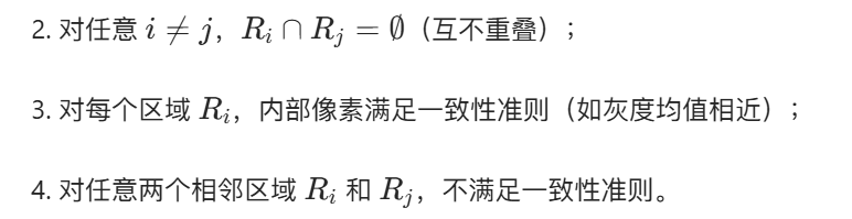
图像分割是将数字图像划分为互不重叠的像素子集 (区域)的过程,分割后的每个区域都具有某种一致性特征(如灰度、颜色、纹理、形状等),而不同区域之间的特征存在显著差异。
10.1.2 分割的本质
从数学角度,设图像为 I(x,y),分割就是找到一组区域 R1,R2,...,Rn,满足:
1.整个图像区域(全覆盖);
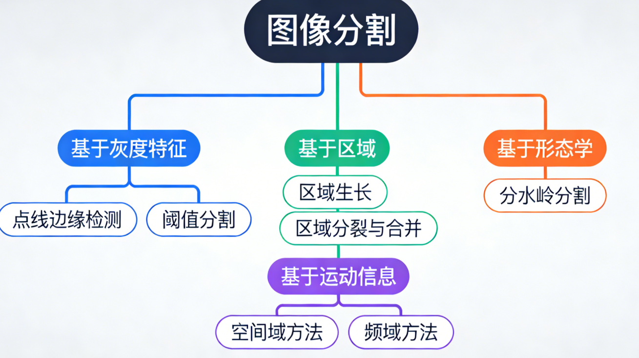
10.1.3 分割方法分类
10.2 点、线与边缘检测
10.2.1 背景知识
点、线、边缘是图像中最基础的灰度突变特征:
- 孤立点:局部区域内灰度值与周围像素差异极大的单个像素;
- 线:由一系列相邻的、灰度突变的像素组成的一维结构;
- 边缘:图像中灰度、颜色、纹理等特征发生突变的像素集合,是区域的边界。
10.2.2 孤立点检测
原理
通过邻域灰度差检测孤立点:计算像素在 n×n 邻域内的灰度最大值 / 最小值与该像素的差值,若差值超过设定阈值,则判定为孤立点。常用 3×3 邻域,核心公式:
完整代码(含效果对比)
import cv2
import numpy as np
import matplotlib.pyplot as plt

# 设置matplotlib支持中文显示
plt.rcParams['font.sans-serif'] = ['SimHei']  # 黑体
plt.rcParams['axes.unicode_minus'] = False    # 解决负号显示问题

def detect_isolated_points(img, kernel_size=3, threshold=50):
    """
    孤立点检测
    :param img: 输入灰度图像
    :param kernel_size: 邻域大小(奇数)
    :param threshold: 灰度差阈值
    :return: 标记孤立点的图像
    """
    # 生成邻域均值图像
    kernel = np.ones((kernel_size, kernel_size), np.float32) / (kernel_size**2)
    mean_img = cv2.filter2D(img, -1, kernel)

    # 计算灰度差绝对值
    diff = cv2.absdiff(img, mean_img)

    # 阈值化检测孤立点
    _, points_img = cv2.threshold(diff, threshold, 255, cv2.THRESH_BINARY)

    # 将孤立点标记在原图上(红色)
    img_color = cv2.cvtColor(img, cv2.COLOR_GRAY2BGR)
    img_color[points_img == 255] = [0, 0, 255]  # BGR格式,红色

    return points_img, img_color

# 1. 加载图像(转为灰度图)
img = cv2.imread('test_img.jpg', 0)  # 替换为你的图像路径,0表示灰度模式
if img is None:
    # 若加载失败,使用内置测试图像
    img = cv2.imread(cv2.samples.findFile('lena.jpg'), 0)

# 2. 孤立点检测
points_img, marked_img = detect_isolated_points(img, threshold=40)

# 3. 效果对比显示
plt.figure(figsize=(15, 5))
plt.subplot(131)
plt.imshow(img, cmap='gray')
plt.title('原始灰度图像')
plt.axis('off')

plt.subplot(132)
plt.imshow(points_img, cmap='gray')
plt.title('孤立点检测结果')
plt.axis('off')

plt.subplot(133)
plt.imshow(cv2.cvtColor(marked_img, cv2.COLOR_BGR2RGB))
plt.title('标记孤立点的原图')
plt.axis('off')

plt.show()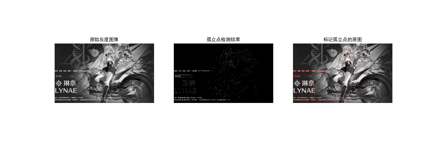
10.2.3 线检测
原理
线检测基于方向模板卷积,常用模板包括水平、垂直、45°、135° 线模板。以 3×3 模板为例:
卷积后,若像素值超过阈值,则判定为对应方向的线。
完整代码(含效果对比)
python
# 导入必要的库
import cv2
import numpy as np
import matplotlib.pyplot as plt

# ===================== 配置项 =====================
# 替换为你自己的图片路径(绝对路径/相对路径均可)
IMAGE_PATH = "../picture/AALi.jpg"  # 例如:"D:/test/road.jpg" 或 "./my_photo.png"
# 线检测阈值(可根据图片效果调整)
LINE_THRESHOLD = 100
# 显示窗口大小
FIG_SIZE = (22, 12)
# ==================================================

# 设置matplotlib支持中文显示(解决标题乱码问题)
plt.rcParams['font.sans-serif'] = ['SimHei']  # 黑体
plt.rcParams['axes.unicode_minus'] = False  # 解决负号显示问题


def detect_lines(img_gray, threshold=100):
    """
    多方向线检测
    :param img_gray: 输入灰度图像
    :param threshold: 线检测阈值
    :return: 各方向线检测结果
    """
    # 定义线检测模板
    horizontal_kernel = np.array([[1, 1, 1], [-1, -1, -1], [-1, -1, -1]], dtype=np.float32)
    vertical_kernel = np.array([[1, -1, -1], [1, -1, -1], [1, -1, -1]], dtype=np.float32)
    diagonal45_kernel = np.array([[-1, -1, 1], [-1, 1, -1], [1, -1, -1]], dtype=np.float32)
    diagonal135_kernel = np.array([[1, -1, -1], [-1, 1, -1], [-1, -1, 1]], dtype=np.float32)

    # 卷积计算(提取各方向线特征)
    horizontal_lines = cv2.filter2D(img_gray, -1, horizontal_kernel)
    vertical_lines = cv2.filter2D(img_gray, -1, vertical_kernel)
    diagonal45_lines = cv2.filter2D(img_gray, -1, diagonal45_kernel)
    diagonal135_lines = cv2.filter2D(img_gray, -1, diagonal135_kernel)

    # 阈值化增强效果(二值化,突出线特征)
    horizontal_lines = cv2.threshold(np.abs(horizontal_lines), threshold, 255, cv2.THRESH_BINARY)[1]
    vertical_lines = cv2.threshold(np.abs(vertical_lines), threshold, 255, cv2.THRESH_BINARY)[1]
    diagonal45_lines = cv2.threshold(np.abs(diagonal45_lines), threshold, 255, cv2.THRESH_BINARY)[1]
    diagonal135_lines = cv2.threshold(np.abs(diagonal135_lines), threshold, 255, cv2.THRESH_BINARY)[1]

    return horizontal_lines, vertical_lines, diagonal45_lines, diagonal135_lines


def main():
    # 1. 加载图像(优先加载自定义图片)
    # 读取彩色原图(cv2默认BGR格式)
    img_color = cv2.imread(IMAGE_PATH)
    if img_color is None:
        print(f"警告:未找到自定义图片 {IMAGE_PATH},使用内置测试图片(lena)")
        img_color = cv2.imread(cv2.samples.findFile('lena.jpg'))

    # 转换为灰度图(用于线检测)
    img_gray = cv2.cvtColor(img_color, cv2.COLOR_BGR2GRAY)

    # 2. 执行多方向线检测
    horizontal, vertical, diagonal45, diagonal135 = detect_lines(img_gray, LINE_THRESHOLD)

    # 3. 合并所有方向的线特征
    all_lines = cv2.addWeighted(horizontal, 0.25, vertical, 0.25, 0)
    all_lines = cv2.addWeighted(all_lines, 1, diagonal45, 0.25, 0)
    all_lines = cv2.addWeighted(all_lines, 1, diagonal135, 0.25, 0)

    # 4. 效果对比显示(同一窗口)
    plt.figure(figsize=FIG_SIZE)

    # 子图1:原始彩色图片(转换为RGB格式显示)
    plt.subplot(2, 4, 1)
    plt.imshow(cv2.cvtColor(img_color, cv2.COLOR_BGR2RGB))
    plt.title('1. 原始彩色图像', fontsize=12)
    plt.axis('off')  # 隐藏坐标轴

    # 子图2:原始灰度图片
    plt.subplot(2, 4, 2)
    plt.imshow(img_gray, cmap='gray')
    plt.title('2. 原始灰度图像', fontsize=12)
    plt.axis('off')

    # 子图3:水平线检测结果
    plt.subplot(2, 4, 3)
    plt.imshow(horizontal, cmap='gray')
    plt.title('3. 水平线检测', fontsize=12)
    plt.axis('off')

    # 子图4:垂直线检测结果
    plt.subplot(2, 4, 4)
    plt.imshow(vertical, cmap='gray')
    plt.title('4. 垂直线检测', fontsize=12)
    plt.axis('off')

    # 子图5:45°线检测结果
    plt.subplot(2, 4, 5)
    plt.imshow(diagonal45, cmap='gray')
    plt.title('5. 45°线检测', fontsize=12)
    plt.axis('off')

    # 子图6:135°线检测结果
    plt.subplot(2, 4, 6)
    plt.imshow(diagonal135, cmap='gray')
    plt.title('6. 135°线检测', fontsize=12)
    plt.axis('off')

    # 子图7:所有方向线合并结果
    plt.subplot(2, 4, 7)
    plt.imshow(all_lines, cmap='gray')
    plt.title('7. 所有方向线合并', fontsize=12)
    plt.axis('off')

    # 子图8:合并线叠加到彩色原图(可视化效果)
    plt.subplot(2, 4, 8)
    img_overlay = img_color.copy()
    img_overlay[all_lines == 255] = [0, 0, 255]  # 线区域标记为红色(BGR)
    plt.imshow(cv2.cvtColor(img_overlay, cv2.COLOR_BGR2RGB))
    plt.title('8. 线检测结果叠加原图', fontsize=12)
    plt.axis('off')

    # 调整子图间距,避免重叠
    plt.tight_layout()
    # 显示所有图片
    plt.show()


if __name__ == "__main__":
    main()
10.2.4 边缘模型
边缘的灰度分布主要有三种模型:
- 阶跃型边缘:灰度从一个值突变到另一个值(如物体边界);
- 斜坡型边缘:灰度从一个值渐变到另一个值(渐变区域);
- 屋顶型边缘:灰度先升后降(细线、条纹)。
数学上,边缘对应灰度函数的一阶导数极值 或二阶导数过零点(拉普拉斯算子)。
10.2.5 基础边缘检测
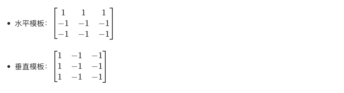
常用算子
- Roberts 算子:基于 2×2 邻域的差分,检测斜向边缘;
- Prewitt 算子:3×3 邻域,分水平 / 垂直方向,抗噪声能力优于 Roberts;
- Sobel 算子:3×3 邻域,带权重的差分,抗噪声能力更强。
完整代码(含效果对比)
python
# 导入必要的库
import cv2
import numpy as np
import matplotlib.pyplot as plt

# ===================== 核心配置项 =====================
# 替换为你自己的图片路径(绝对/相对路径均可)
IMAGE_PATH = "../picture/JinXi.png"  # 示例:"D:/images/road.jpg" 或 "./my_photo.png"
# 显示窗口尺寸(可根据需求调整)
FIG_SIZE = (20, 10)
# ======================================================

# 设置matplotlib支持中文显示(解决标题/标签乱码)
plt.rcParams['font.sans-serif'] = ['SimHei']  # 启用黑体字体
plt.rcParams['axes.unicode_minus'] = False  # 解决负号显示异常


def basic_edge_detection(img_gray):
    """
    基础边缘检测(Roberts/Prewitt/Sobel)
    :param img_gray: 输入灰度图像
    :return: roberts_edge, prewitt_edge, sobel_edge 各算子检测结果
    """
    # ---------------------- Roberts算子 ----------------------
    # 定义Roberts交叉梯度算子(2x2)
    roberts_x = np.array([[1, 0], [0, -1]], dtype=np.float32)
    roberts_y = np.array([[0, 1], [-1, 0]], dtype=np.float32)
    # 卷积计算x/y方向梯度
    roberts_x_edge = cv2.filter2D(img_gray, -1, roberts_x)
    roberts_y_edge = cv2.filter2D(img_gray, -1, roberts_y)
    # 计算梯度幅值(合并x/y方向)
    roberts_edge = cv2.magnitude(roberts_x_edge.astype(np.float32), roberts_y_edge.astype(np.float32))
    # 归一化到0-255并转换为uint8类型
    roberts_edge = np.uint8(np.clip(roberts_edge, 0, 255))

    # ---------------------- Prewitt算子 ----------------------
    # 定义Prewitt算子(3x3,分x/y方向)
    prewitt_x = np.array([[-1, 0, 1], [-1, 0, 1], [-1, 0, 1]], dtype=np.float32)  # 水平梯度
    prewitt_y = np.array([[-1, -1, -1], [0, 0, 0], [1, 1, 1]], dtype=np.float32)  # 垂直梯度
    # 卷积计算x/y方向梯度
    prewitt_x_edge = cv2.filter2D(img_gray, -1, prewitt_x)
    prewitt_y_edge = cv2.filter2D(img_gray, -1, prewitt_y)
    # 计算梯度幅值
    prewitt_edge = cv2.magnitude(prewitt_x_edge.astype(np.float32), prewitt_y_edge.astype(np.float32))
    prewitt_edge = np.uint8(np.clip(prewitt_edge, 0, 255))

    # ---------------------- Sobel算子 ----------------------
    # Sobel算子(OpenCV内置函数,精度更高)
    sobel_x = cv2.Sobel(img_gray, cv2.CV_64F, 1, 0, ksize=3)  # x方向梯度(dx=1, dy=0)
    sobel_y = cv2.Sobel(img_gray, cv2.CV_64F, 0, 1, ksize=3)  # y方向梯度(dx=0, dy=1)
    # 计算梯度幅值
    sobel_edge = cv2.magnitude(sobel_x, sobel_y)
    sobel_edge = np.uint8(np.clip(sobel_edge, 0, 255))

    return roberts_edge, prewitt_edge, sobel_edge


def main():
    # 1. 加载图像(优先使用自定义图片)
    # 读取彩色原图(cv2默认BGR格式,需转换为RGB用于matplotlib显示)
    img_color = cv2.imread(IMAGE_PATH)
    if img_color is None:
        print(f"警告:未找到自定义图片 {IMAGE_PATH},自动使用内置测试图片(Lena)")
        img_color = cv2.imread(cv2.samples.findFile('lena.jpg'))

    # 转换为灰度图(边缘检测的输入要求)
    img_gray = cv2.cvtColor(img_color, cv2.COLOR_BGR2GRAY)

    # 2. 执行基础边缘检测
    roberts, prewitt, sobel = basic_edge_detection(img_gray)

    # 3. 效果对比可视化(同一窗口展示所有结果)
    plt.figure(figsize=FIG_SIZE)

    # 子图1:原始彩色图片
    plt.subplot(2, 3, 1)
    plt.imshow(cv2.cvtColor(img_color, cv2.COLOR_BGR2RGB))
    plt.title('1. 原始彩色图像', fontsize=12)
    plt.axis('off')  # 隐藏坐标轴

    # 子图2:原始灰度图片
    plt.subplot(2, 3, 2)
    plt.imshow(img_gray, cmap='gray')
    plt.title('2. 原始灰度图像', fontsize=12)
    plt.axis('off')

    # 子图3:Roberts算子检测结果
    plt.subplot(2, 3, 3)
    plt.imshow(roberts, cmap='gray')
    plt.title('3. Roberts算子', fontsize=12)
    plt.axis('off')

    # 子图4:Prewitt算子检测结果
    plt.subplot(2, 3, 4)
    plt.imshow(prewitt, cmap='gray')
    plt.title('4. Prewitt算子', fontsize=12)
    plt.axis('off')

    # 子图5:Sobel算子检测结果
    plt.subplot(2, 3, 5)
    plt.imshow(sobel, cmap='gray')
    plt.title('5. Sobel算子', fontsize=12)
    plt.axis('off')

    # 子图6:Sobel边缘叠加到彩色原图(增强可视化效果)
    plt.subplot(2, 3, 6)
    img_overlay = img_color.copy()
    img_overlay[sobel > 50] = [0, 0, 255]  # 边缘区域标记为红色(BGR格式)
    plt.imshow(cv2.cvtColor(img_overlay, cv2.COLOR_BGR2RGB))
    plt.title('6. Sobel边缘叠加原图', fontsize=12)
    plt.axis('off')

    # 调整子图间距,避免标题/图片重叠
    plt.tight_layout()
    # 显示所有子图
    plt.show()


# 程序入口
if __name__ == "__main__":
    main()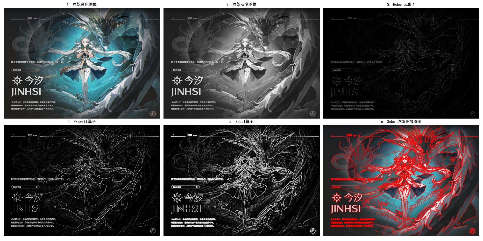
10.2.6 高级边缘检测技术
Canny 边缘检测(工业级标准)
Canny 边缘检测是目前最常用的高级边缘检测算法,核心步骤:
- 高斯平滑:去除噪声;
- 计算梯度幅值和方向:用 Sobel 算子计算;
- 非极大值抑制:保留梯度方向上的局部最大值,细化边缘;
- 双阈值检测:区分强边缘、弱边缘,仅保留强边缘和连接强边缘的弱边缘。
完整代码(含效果对比)
python
# 导入必要的库
import cv2
import numpy as np
import matplotlib.pyplot as plt
import os  # 新增:处理路径兼容性

IMAGE_PATH = "../picture/KanTeLeiLa.png"

# Canny检测的三组阈值(可根据图片效果调整)
CANNY_THRESHOLDS = [
    (30, 90),  # 低阈值组合
    (50, 150),  # 中等阈值组合
    (80, 200)  # 高阈值组合
]
# 显示窗口尺寸
FIG_SIZE = (22, 10)
# ======================================================

# 修复字体警告:使用支持更多符号的中文字体,优先系统自带字体
plt.rcParams['font.sans-serif'] = ['Microsoft YaHei', 'SimHei', 'DejaVu Sans']  # 增加备选字体
plt.rcParams['axes.unicode_minus'] = False
plt.rcParams['font.family'] = 'sans-serif'  # 明确字体族


def canny_edge_detection(img_gray, low_threshold=50, high_threshold=150):
    """
    Canny边缘检测(工业级标准边缘检测算法)
    :param img_gray: 输入灰度图像
    :param low_threshold: 双阈值检测的低阈值(弱边缘判定)
    :param high_threshold: 双阈值检测的高阈值(强边缘判定)
    :return: Canny边缘检测结果(二值图)
    """
    # 步骤1:高斯平滑(去除噪声,提升边缘检测稳定性)
    blur_img = cv2.GaussianBlur(img_gray, (3, 3), 1)  # 3x3高斯核,标准差1
    # 步骤2:Canny边缘检测(内置:梯度计算→非极大值抑制→双阈值检测→边缘连接)
    canny_edge = cv2.Canny(blur_img, low_threshold, high_threshold)
    return canny_edge


def main():
    # 1. 加载图像(优先使用自定义图片,失败则降级到内置测试图)
    # 检查路径是否存在,增加容错提示
    if not os.path.exists(IMAGE_PATH):
        print(f"警告:图片路径 {IMAGE_PATH} 不存在!")
        img_color = None
    else:
        img_color = cv2.imread(IMAGE_PATH)

    if img_color is None:
        print(f"自动使用内置测试图片(Lena)")
        img_color = cv2.imread(cv2.samples.findFile('lena.jpg'))

    # 转换为灰度图(Canny检测要求输入灰度图)
    img_gray = cv2.cvtColor(img_color, cv2.COLOR_BGR2GRAY)

    # 2. 执行不同阈值的Canny边缘检测
    canny_results = []
    for idx, (low, high) in enumerate(CANNY_THRESHOLDS):
        canny_edge = canny_edge_detection(img_gray, low, high)
        canny_results.append((low, high, canny_edge))

    # 3. 效果对比可视化(同一窗口展示所有结果)
    plt.figure(figsize=FIG_SIZE)

    # 子图1:原始彩色图片
    plt.subplot(2, 4, 1)
    plt.imshow(cv2.cvtColor(img_color, cv2.COLOR_BGR2RGB))
    plt.title('1. 原始彩色图像', fontsize=12)
    plt.axis('off')  # 隐藏坐标轴

    # 子图2:原始灰度图片
    plt.subplot(2, 4, 2)
    plt.imshow(img_gray, cmap='gray')
    plt.title('2. 原始灰度图像', fontsize=12)
    plt.axis('off')

    # 子图3-5:不同阈值的Canny检测结果
    for idx, (low, high, edge) in enumerate(canny_results):
        plt.subplot(2, 4, idx + 3)
        plt.imshow(edge, cmap='gray')
        plt.title(f'{idx + 3}. Canny({low},{high}) - {"低" if idx == 0 else "中等" if idx == 1 else "高"}阈值',
                  fontsize=11)
        plt.axis('off')

    # 子图6:最优阈值(中等)边缘叠加到彩色原图(增强可视化)
    plt.subplot(2, 4, 7)
    img_overlay = img_color.copy()
    mid_edge = canny_results[1][2]  # 取中等阈值的检测结果
    img_overlay[mid_edge > 0] = [0, 0, 255]  # 边缘区域标记为红色(BGR格式)
    plt.imshow(cv2.cvtColor(img_overlay, cv2.COLOR_BGR2RGB))
    plt.title('7. 中等阈值边缘叠加原图', fontsize=12)
    plt.axis('off')

    # 子图7:阈值对比说明(替换圆点为中文符号,彻底解决字体警告)
    plt.subplot(2, 4, 8)
    # 把•换成中文全角的·,避免字体缺失问题
    plt.text(0.1, 0.8, '阈值说明:\n· 低阈值:检测更多边缘(含噪声)\n· 中等阈值:平衡边缘与噪声\n· 高阈值:仅保留强边缘',
             fontsize=11, verticalalignment='top', fontfamily='sans-serif')
    plt.axis('off')  # 隐藏坐标轴
    plt.xticks([])
    plt.yticks([])

    # 调整子图间距,避免标题/图片重叠
    plt.tight_layout()
    # 显示所有子图
    plt.show()


# 程序入口
if __name__ == "__main__":
    main()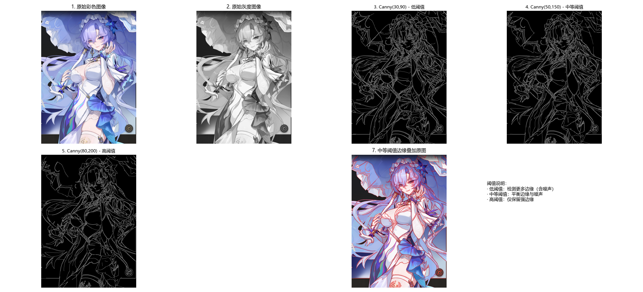
10.2.7 边缘连接与边界检测
边缘连接的核心是将离散的边缘点连接成连续的边界,常用方法:
- 基于灰度和梯度的连接:判断相邻边缘点的灰度、梯度方向是否一致;
- 霍夫变换:检测直线 / 曲线边界(如圆形、椭圆)。
霍夫直线检测代码(边界检测示例)
python
# 导入必要的库
import cv2
import numpy as np
import matplotlib.pyplot as plt
import os  # 处理路径兼容性

# ===================== 核心配置项 =====================
# 替换为你自己的图片路径(绝对/相对路径均可)
# 推荐使用含直线的图片:棋盘格、道路、建筑、表格等
IMAGE_PATH = r"../picture/GaoDa.png"  # Windows示例:r"D:\images\chessboard.png"
# 霍夫直线检测参数(可根据图片效果调整)
HOUGH_PARAMS = {
    "canny_low": 50,  # Canny低阈值
    "canny_high": 150,  # Canny高阈值
    "threshold": 80,  # 霍夫检测阈值(越高检测越少直线)
    "minLineLength": 30,  # 最小直线长度(短于该值的线忽略)
    "maxLineGap": 10  # 最大线段间隙(间隙内的线段合并为一条)
}
# 显示窗口尺寸
FIG_SIZE = (18, 8)
# ======================================================

# 设置matplotlib支持中文显示(解决标题乱码+特殊符号警告)
plt.rcParams['font.sans-serif'] = ['Microsoft YaHei', 'SimHei', 'DejaVu Sans']
plt.rcParams['axes.unicode_minus'] = False
plt.rcParams['font.family'] = 'sans-serif'


def hough_line_detection(img_gray, canny_low=50, canny_high=150, threshold=80, minLineLength=30, maxLineGap=10):
    """
    霍夫直线检测(边缘连接+边界检测)
    :param img_gray: 输入灰度图像
    :param canny_low: Canny边缘检测低阈值
    :param canny_high: Canny边缘检测高阈值
    :param threshold: 霍夫直线检测阈值
    :param minLineLength: 最小直线长度
    :param maxLineGap: 最大线段间隙
    :return: canny_edge(Canny边缘图), line_img(标记直线的彩色图)
    """
    # 步骤1:Canny边缘检测(提取图像边缘,为霍夫检测做准备)
    canny_edge = cv2.Canny(img_gray, canny_low, canny_high)

    # 步骤2:概率霍夫直线检测(HoughLinesP:效率更高,直接返回线段端点)
    # 参数说明:
    # 1: 距离分辨率(像素);np.pi/180: 角度分辨率(弧度)
    # threshold: 累加器阈值(只有投票数超过该值才被认为是直线)
    # minLineLength: 最小直线长度;maxLineGap: 同一线的最大像素间隙
    lines = cv2.HoughLinesP(
        canny_edge,
        1, np.pi / 180,
        threshold=threshold,
        minLineLength=minLineLength,
        maxLineGap=maxLineGap
    )

    # 步骤3:在灰度图转彩色的图像上绘制检测到的直线(红色)
    img_color = cv2.cvtColor(img_gray, cv2.COLOR_GRAY2BGR)
    if lines is not None:
        for line in lines:
            x1, y1, x2, y2 = line[0]
            cv2.line(img_color, (x1, y1), (x2, y2), (0, 0, 255), 2)  # 红色,线宽2

    return canny_edge, img_color


def main():
    # 1. 加载图像(优先使用自定义图片,失败则降级到内置测试图)
    # 检查路径是否存在,增加容错提示
    if not os.path.exists(IMAGE_PATH):
        print(f"警告:图片路径 {IMAGE_PATH} 不存在!")
        img_color = None
    else:
        img_color = cv2.imread(IMAGE_PATH)  # 读取彩色原图

    if img_color is None:
        print(f"自动使用内置测试图片(棋盘格)")
        img_color = cv2.imread(cv2.samples.findFile('chessboard.png'))

    # 转换为灰度图(霍夫检测要求输入灰度图)
    img_gray = cv2.cvtColor(img_color, cv2.COLOR_BGR2GRAY)

    # 2. 执行霍夫直线检测
    canny_edge, line_img = hough_line_detection(
        img_gray,
        canny_low=HOUGH_PARAMS["canny_low"],
        canny_high=HOUGH_PARAMS["canny_high"],
        threshold=HOUGH_PARAMS["threshold"],
        minLineLength=HOUGH_PARAMS["minLineLength"],
        maxLineGap=HOUGH_PARAMS["maxLineGap"]
    )

    # 3. 效果对比可视化(同一窗口展示所有结果)
    plt.figure(figsize=FIG_SIZE)

    # 子图1:原始彩色图片
    plt.subplot(2, 2, 1)
    plt.imshow(cv2.cvtColor(img_color, cv2.COLOR_BGR2RGB))
    plt.title('1. 原始彩色图像', fontsize=12)
    plt.axis('off')  # 隐藏坐标轴

    # 子图2:原始灰度图片
    plt.subplot(2, 2, 2)
    plt.imshow(img_gray, cmap='gray')
    plt.title('2. 原始灰度图像', fontsize=12)
    plt.axis('off')

    # 子图3:Canny边缘检测结果(霍夫检测的输入)
    plt.subplot(2, 2, 3)
    plt.imshow(canny_edge, cmap='gray')
    plt.title('3. Canny边缘检测', fontsize=12)
    plt.axis('off')

    # 子图4:霍夫直线检测结果(红色标记直线)
    plt.subplot(2, 2, 4)
    plt.imshow(cv2.cvtColor(line_img, cv2.COLOR_BGR2RGB))
    plt.title('4. 霍夫直线检测(边界连接)', fontsize=12)
    plt.axis('off')

    # 调整子图间距,避免标题/图片重叠
    plt.tight_layout()
    # 显示所有子图
    plt.show()


# 程序入口
if __name__ == "__main__":
    main()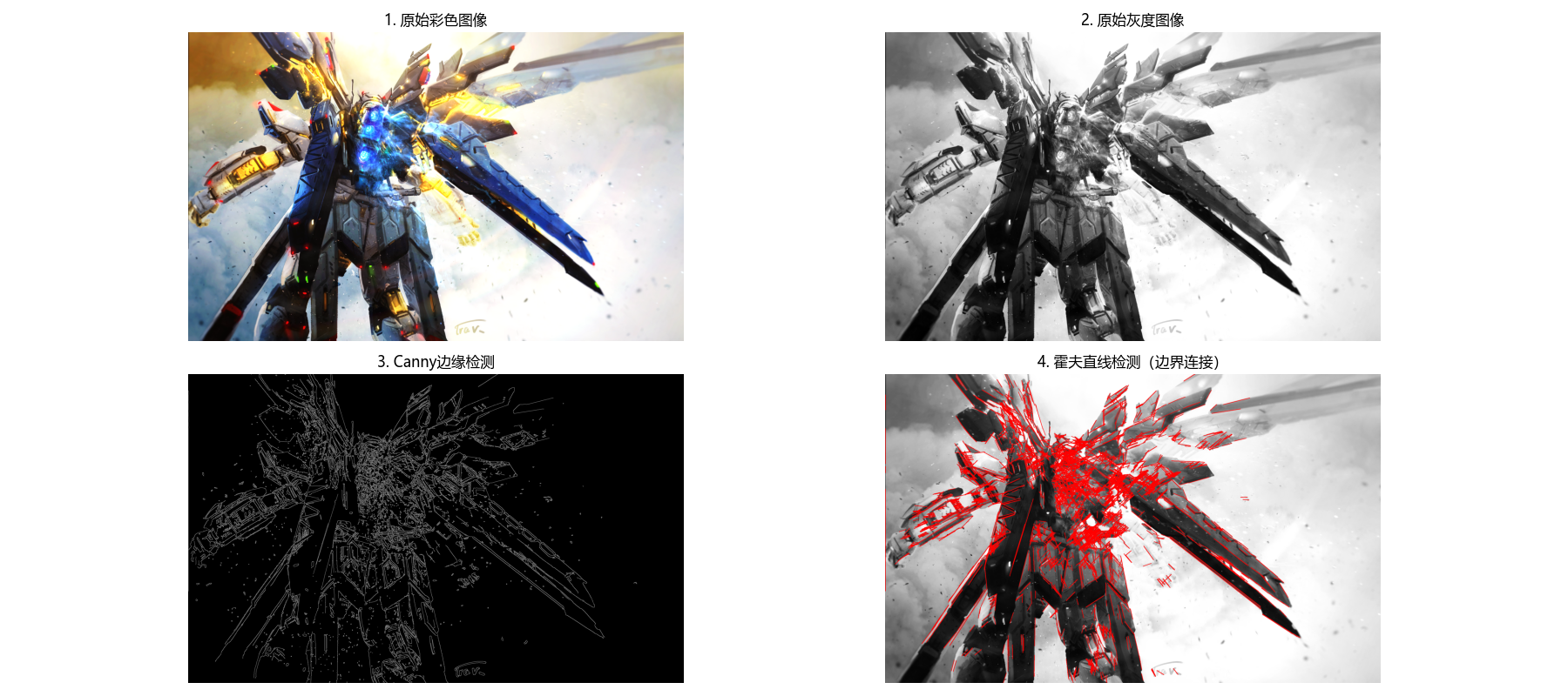
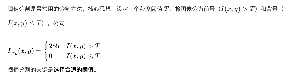
10.3 阈值分割
10.3.1 理论基础
10.3.2 基础全局阈值分割
全局阈值:整幅图像使用同一个阈值,适用于前景和背景灰度分布差异明显的图像。
完整代码(含效果对比)
python
# 导入必要的库
import cv2
import numpy as np
import matplotlib.pyplot as plt
import os  # 处理路径兼容性

# ===================== 核心配置项 =====================
# 替换为你自己的图片路径(绝对/相对路径均可)
IMAGE_PATH = r"../picture/AoGuSiTa.png"  # Windows示例:r"D:\images\test.png"
# 全局阈值分割的三组阈值(可根据图片效果调整)
GLOBAL_THRESHOLDS = [80, 127, 180]  # 低/默认/高阈值
# 显示窗口尺寸
FIG_SIZE = (22, 10)
# ======================================================

# 设置matplotlib支持中文显示(解决标题乱码+特殊符号警告)
plt.rcParams['font.sans-serif'] = ['Microsoft YaHei', 'SimHei', 'DejaVu Sans']
plt.rcParams['axes.unicode_minus'] = False
plt.rcParams['font.family'] = 'sans-serif'


def global_threshold_segmentation(img_gray, threshold=127):
    """
    基础全局阈值分割(二值化)
    :param img_gray: 输入灰度图像(0-255)
    :param threshold: 全局阈值(0-255)
    :return: 分割结果(二值图:大于阈值为255(白),小于等于为0(黑))
    """
    # cv2.threshold参数说明:
    # img_gray: 输入灰度图;threshold: 阈值;255: 最大值(超过阈值的像素设为该值)
    # cv2.THRESH_BINARY: 二值化模式(>threshold→255,≤threshold→0)
    _, seg_img = cv2.threshold(img_gray, threshold, 255, cv2.THRESH_BINARY)
    return seg_img


def main():
    # 1. 加载图像(优先使用自定义图片,失败则降级到内置测试图)
    # 检查路径是否存在,增加容错提示
    if not os.path.exists(IMAGE_PATH):
        print(f"警告:图片路径 {IMAGE_PATH} 不存在!")
        img_color = None
    else:
        img_color = cv2.imread(IMAGE_PATH)  # 读取彩色原图

    if img_color is None:
        print(f"自动使用内置测试图片(Lena)")
        img_color = cv2.imread(cv2.samples.findFile('lena.jpg'))

    # 转换为灰度图(阈值分割要求输入灰度图)
    img_gray = cv2.cvtColor(img_color, cv2.COLOR_BGR2GRAY)

    # 2. 执行不同阈值的全局分割
    seg_results = []
    for threshold in GLOBAL_THRESHOLDS:
        seg_img = global_threshold_segmentation(img_gray, threshold)
        seg_results.append((threshold, seg_img))

    # 3. 效果对比可视化(同一窗口展示所有结果)
    plt.figure(figsize=FIG_SIZE)

    # 子图1:原始彩色图片
    plt.subplot(2, 4, 1)
    plt.imshow(cv2.cvtColor(img_color, cv2.COLOR_BGR2RGB))
    plt.title('1. 原始彩色图像', fontsize=12)
    plt.axis('off')  # 隐藏坐标轴

    # 子图2:原始灰度图片
    plt.subplot(2, 4, 2)
    plt.imshow(img_gray, cmap='gray')
    plt.title('2. 原始灰度图像', fontsize=12)
    plt.axis('off')

    # 子图3-5:不同阈值的分割结果
    for idx, (threshold, seg_img) in enumerate(seg_results):
        plt.subplot(2, 4, idx + 3)
        plt.imshow(seg_img, cmap='gray')
        threshold_desc = "低阈值" if idx == 0 else "默认阈值" if idx == 1 else "高阈值"
        plt.title(f'{idx + 3}. 阈值={threshold}({threshold_desc})', fontsize=11)
        plt.axis('off')

    # 子图6:阈值分割原理说明(辅助理解)
    plt.subplot(2, 4, 7)
    # 计算灰度直方图(直观展示阈值分割的依据)
    hist = cv2.calcHist([img_gray], [0], None, [256], [0, 256])
    plt.plot(hist, color='black')
    # 标记三组阈值线
    colors = ['red', 'green', 'blue']
    for i, threshold in enumerate(GLOBAL_THRESHOLDS):
        plt.axvline(x=threshold, color=colors[i], linestyle='--', label=f'阈值={threshold}')
    plt.xlim([0, 255])
    plt.xlabel('灰度值')
    plt.ylabel('像素数量')
    plt.title('7. 灰度直方图+阈值标记', fontsize=11)
    plt.legend(fontsize=9)

    # 子图7:阈值分割效果总结
    plt.subplot(2, 4, 8)
    plt.text(0.1, 0.8,
             '阈值分割总结:\n· 低阈值(80):更多区域为白色\n· 中阈值(127):平衡黑白分布\n· 高阈值(180):更多区域为黑色',
             fontsize=11, verticalalignment='top', fontfamily='sans-serif')
    plt.axis('off')
    plt.xticks([])
    plt.yticks([])

    # 调整子图间距,避免标题/图片重叠
    plt.tight_layout()
    # 显示所有子图
    plt.show()


# 程序入口
if __name__ == "__main__":
    main()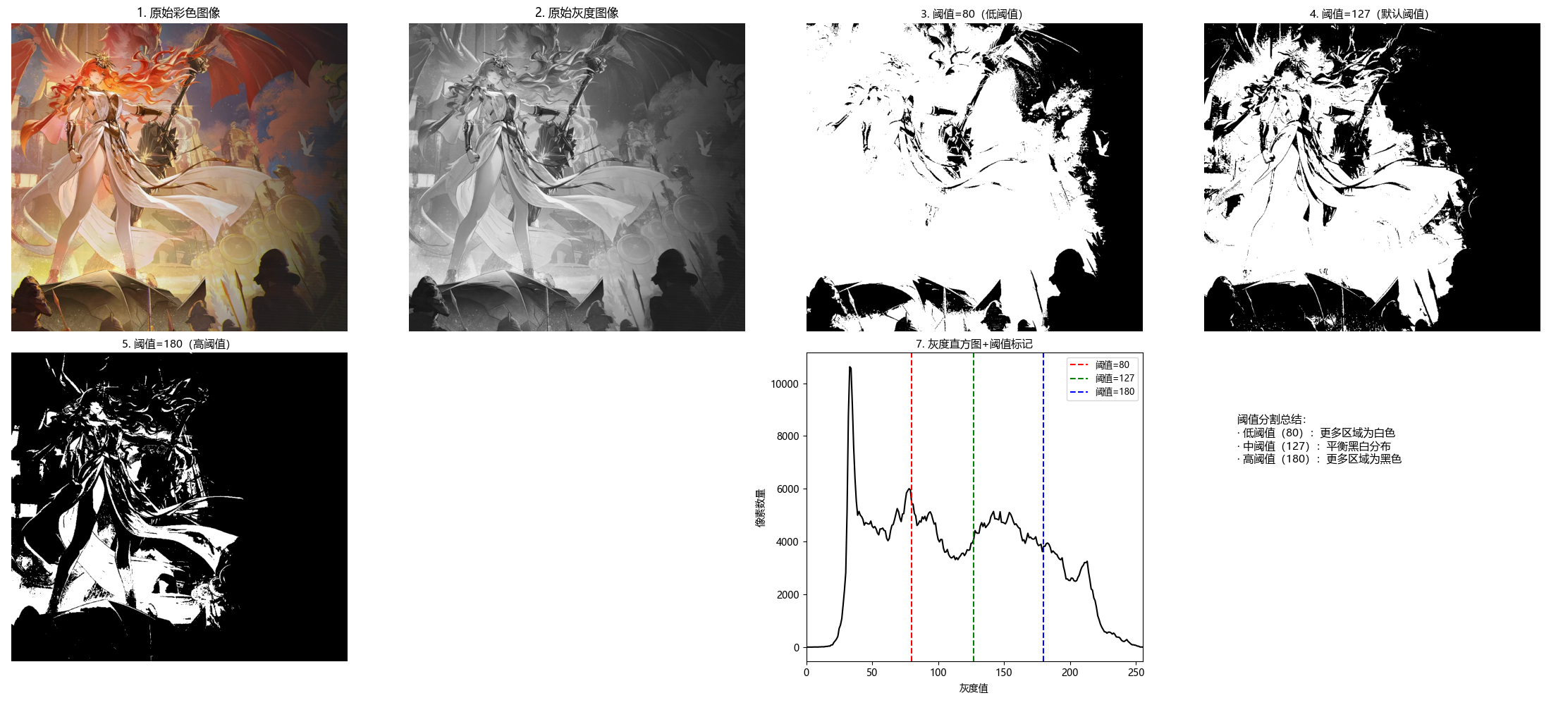
10.3.3 基于大津法的最优全局阈值分割
完整代码(含效果对比)
python
# 导入必要的库
import cv2
import numpy as np
import matplotlib.pyplot as plt
import os  # 处理路径兼容性

# ===================== 核心配置项 =====================
# 替换为你自己的图片路径(绝对/相对路径均可)
IMAGE_PATH = r"../picture/ShouAnRen.png"  # Windows示例:r"D:\images\test.png"
# 手动对比的阈值(可调整)
MANUAL_THRESHOLD = 127
# 显示窗口尺寸
FIG_SIZE = (20, 10)
# ======================================================

# 设置matplotlib支持中文显示(解决标题乱码+特殊符号警告)
plt.rcParams['font.sans-serif'] = ['Microsoft YaHei', 'SimHei', 'DejaVu Sans']
plt.rcParams['axes.unicode_minus'] = False
plt.rcParams['font.family'] = 'sans-serif'


def global_threshold_segmentation(img_gray, threshold=127):
    """
    基础全局阈值分割(补充该函数,确保代码独立运行)
    :param img_gray: 输入灰度图像
    :param threshold: 全局阈值
    :return: 二值化分割结果
    """
    _, seg_img = cv2.threshold(img_gray, threshold, 255, cv2.THRESH_BINARY)
    return seg_img


def otsu_threshold_segmentation(img_gray):
    """
    大津法(OTSU)最优阈值分割
    原理:自动计算使类间方差最大的阈值,适用于双峰灰度分布的图像
    :param img_gray: 输入灰度图像
    :return: seg_img(分割结果), optimal_threshold(自动计算的最优阈值)
    """
    # cv2.THRESH_OTSU:自动计算最优阈值(此时第一个参数threshold设为0即可)
    optimal_threshold, seg_img = cv2.threshold(
        img_gray,
        0, 255,
        cv2.THRESH_BINARY + cv2.THRESH_OTSU
    )
    return seg_img, optimal_threshold


def main():
    # 1. 加载图像(优先使用自定义图片,失败则降级到内置测试图)
    # 检查路径是否存在,增加容错提示
    if not os.path.exists(IMAGE_PATH):
        print(f"警告:图片路径 {IMAGE_PATH} 不存在!")
        img_color = None
    else:
        img_color = cv2.imread(IMAGE_PATH)  # 读取彩色原图

    if img_color is None:
        print(f"自动使用内置测试图片(Lena)")
        img_color = cv2.imread(cv2.samples.findFile('lena.jpg'))

    # 转换为灰度图(阈值分割要求输入灰度图)
    img_gray = cv2.cvtColor(img_color, cv2.COLOR_BGR2GRAY)

    # 2. 执行阈值分割
    # 大津法自动分割(获取最优阈值和结果)
    otsu_seg, otsu_thresh = otsu_threshold_segmentation(img_gray)
    # 手动阈值分割(对比组)
    manual_seg = global_threshold_segmentation(img_gray, MANUAL_THRESHOLD)

    # 3. 效果对比可视化(同一窗口展示所有结果)
    plt.figure(figsize=FIG_SIZE)

    # 子图1:原始彩色图片
    plt.subplot(2, 3, 1)
    plt.imshow(cv2.cvtColor(img_color, cv2.COLOR_BGR2RGB))
    plt.title('1. 原始彩色图像', fontsize=12)
    plt.axis('off')  # 隐藏坐标轴

    # 子图2:原始灰度图片
    plt.subplot(2, 3, 2)
    plt.imshow(img_gray, cmap='gray')
    plt.title('2. 原始灰度图像', fontsize=12)
    plt.axis('off')

    # 子图3:手动阈值分割结果
    plt.subplot(2, 3, 3)
    plt.imshow(manual_seg, cmap='gray')
    plt.title(f'3. 手动阈值分割(阈值={MANUAL_THRESHOLD})', fontsize=11)
    plt.axis('off')

    # 子图4:大津法分割结果
    plt.subplot(2, 3, 4)
    plt.imshow(otsu_seg, cmap='gray')
    plt.title(f'4. 大津法分割(最优阈值={otsu_thresh:.1f})', fontsize=11)
    plt.axis('off')

    # 子图5:灰度直方图(标记手动阈值和大津法最优阈值)
    plt.subplot(2, 3, 5)
    # 计算灰度直方图
    hist = cv2.calcHist([img_gray], [0], None, [256], [0, 256])
    plt.plot(hist, color='black', label='灰度直方图')
    # 标记手动阈值(红色虚线)
    plt.axvline(x=MANUAL_THRESHOLD, color='red', linestyle='--', label=f'手动阈值={MANUAL_THRESHOLD}')
    # 标记大津法最优阈值(绿色实线)
    plt.axvline(x=otsu_thresh, color='green', linestyle='-', linewidth=2, label=f'OTSU阈值={otsu_thresh:.1f}')
    plt.xlim([0, 255])
    plt.xlabel('灰度值')
    plt.ylabel('像素数量')
    plt.title('5. 灰度直方图+阈值标记', fontsize=11)
    plt.legend(fontsize=9)

    # 子图6:大津法原理说明
    plt.subplot(2, 3, 6)
    plt.text(0.1, 0.8,
             '大津法(OTSU)核心:\n· 自动计算使「类间方差」最大的阈值\n· 无需手动调参,适配双峰灰度分布图像\n· 对比手动阈值:更贴合图像实际灰度特征',
             fontsize=11, verticalalignment='top', fontfamily='sans-serif')
    plt.axis('off')
    plt.xticks([])
    plt.yticks([])

    # 调整子图间距,避免标题/图片重叠
    plt.tight_layout()
    # 显示所有子图
    plt.show()


# 程序入口
if __name__ == "__main__":
    main()
10.3.4 利用图像平滑改进全局阈值分割
噪声会导致阈值分割结果出现伪影,通过高斯平滑去除噪声后再分割,可显著提升效果。
完整代码(含效果对比)
python
# 导入必要的库
import cv2
import numpy as np
import matplotlib.pyplot as plt
import os  # 处理路径兼容性

# ===================== 核心配置项 =====================
# 替换为你自己的图片路径(绝对/相对路径均可)
IMAGE_PATH = r"../picture/QianXiao.png"  # Windows示例:r"D:\images\test.png"
# 噪声配置(可调整强度)
NOISE_MEAN = 0  # 高斯噪声均值(通常为0)
NOISE_STD = 20  # 高斯噪声标准差(越大噪声越强)
# 高斯平滑配置
BLUR_KERNEL = (5, 5)  # 平滑核大小(奇数,越大平滑越强)
BLUR_SIGMA = 1  # 平滑标准差
# 显示窗口尺寸
FIG_SIZE = (22, 10)
# ======================================================

# 设置matplotlib支持中文显示(解决标题乱码+特殊符号警告)
plt.rcParams['font.sans-serif'] = ['Microsoft YaHei', 'SimHei', 'DejaVu Sans']
plt.rcParams['axes.unicode_minus'] = False
plt.rcParams['font.family'] = 'sans-serif'


def smooth_threshold_segmentation(img_gray, blur_kernel=(5, 5), blur_sigma=1):
    """
    平滑+阈值分割(改进噪声场景下的分割效果)
    :param img_gray: 输入含噪声的灰度图像
    :param blur_kernel: 高斯平滑核大小(奇数)
    :param blur_sigma: 高斯平滑标准差
    :return: seg_original(直接OTSU分割结果), seg_smooth(平滑后OTSU分割结果)
    """
    # 1. 直接对含噪声图像做OTSU分割(对比组,保留噪声影响)
    _, seg_original = cv2.threshold(img_gray, 0, 255, cv2.THRESH_BINARY + cv2.THRESH_OTSU)

    # 2. 高斯平滑(核心步骤:去除高斯噪声,保留边缘)
    # 原理:用邻域像素的加权平均替代当前像素,降低噪声干扰
    blur_img = cv2.GaussianBlur(img_gray, blur_kernel, blur_sigma)

    # 3. 对平滑后的图像做OTSU分割(改进组)
    _, seg_smooth = cv2.threshold(blur_img, 0, 255, cv2.THRESH_BINARY + cv2.THRESH_OTSU)

    return seg_original, seg_smooth


def add_gaussian_noise(img_gray, mean=0, std=20):
    """
    为灰度图像添加高斯噪声(模拟真实场景的噪声干扰)
    :param img_gray: 输入灰度图像
    :param mean: 噪声均值
    :param std: 噪声标准差(越大噪声越明显)
    :return: 含噪声的灰度图像
    """
    # 生成高斯噪声(与原图同尺寸,浮点型)
    noise = np.random.normal(mean, std, img_gray.shape).astype(np.float32)
    # 将噪声叠加到原图(避免溢出,先转浮点再计算)
    noisy_img = img_gray.astype(np.float32) + noise
    # 裁剪到0-255范围并转回uint8类型
    noisy_img = np.clip(noisy_img, 0, 255).astype(np.uint8)
    return noisy_img


def main():
    # 1. 加载图像(优先使用自定义图片,失败则降级到内置测试图)
    # 检查路径是否存在,增加容错提示
    if not os.path.exists(IMAGE_PATH):
        print(f"警告:图片路径 {IMAGE_PATH} 不存在!")
        img_color = None
    else:
        img_color = cv2.imread(IMAGE_PATH)  # 读取彩色原图

    if img_color is None:
        print(f"自动使用内置测试图片(Lena)")
        img_color = cv2.imread(cv2.samples.findFile('lena.jpg'))

    # 转换为灰度图(阈值分割要求输入灰度图)
    img_gray = cv2.cvtColor(img_color, cv2.COLOR_BGR2GRAY)

    # 2. 添加高斯噪声(模拟噪声场景)
    noisy_img = add_gaussian_noise(img_gray, mean=NOISE_MEAN, std=NOISE_STD)

    # 3. 执行平滑+阈值分割
    seg_original, seg_smooth = smooth_threshold_segmentation(
        noisy_img,
        blur_kernel=BLUR_KERNEL,
        blur_sigma=BLUR_SIGMA
    )

    # 4. 效果对比可视化(同一窗口展示所有结果)
    plt.figure(figsize=FIG_SIZE)

    # 子图1:原始彩色图片(无噪声)
    plt.subplot(2, 3, 1)
    plt.imshow(cv2.cvtColor(img_color, cv2.COLOR_BGR2RGB))
    plt.title('1. 原始彩色图像(无噪声)', fontsize=12)
    plt.axis('off')  # 隐藏坐标轴

    # 子图2:原始灰度图片(无噪声)
    plt.subplot(2, 3, 2)
    plt.imshow(img_gray, cmap='gray')
    plt.title('2. 原始灰度图像(无噪声)', fontsize=12)
    plt.axis('off')

    # 子图3:含噪声的灰度图像
    plt.subplot(2, 3, 3)
    plt.imshow(noisy_img, cmap='gray')
    plt.title(f'3. 含高斯噪声的图像(标准差={NOISE_STD})', fontsize=11)
    plt.axis('off')

    # 子图4:直接OTSU分割(噪声影响明显)
    plt.subplot(2, 3, 4)
    plt.imshow(seg_original, cmap='gray')
    plt.title('4. 直接OTSU分割(噪声干扰)', fontsize=11)
    plt.axis('off')

    # 子图5:平滑后OTSU分割(噪声减少,效果改进)
    plt.subplot(2, 3, 5)
    plt.imshow(seg_smooth, cmap='gray')
    plt.title(f'5. 高斯平滑后OTSU分割(核={BLUR_KERNEL})', fontsize=11)
    plt.axis('off')

    # 子图6:方法对比说明
    plt.subplot(2, 3, 6)
    plt.text(0.1, 0.8,
             '降噪+分割核心逻辑:\n· 噪声会导致OTSU分割出现大量伪边缘\n· 高斯平滑:去除噪声,保留主体边缘\n· 平滑后分割:伪边缘减少,结果更清晰',
             fontsize=11, verticalalignment='top', fontfamily='sans-serif')
    plt.axis('off')
    plt.xticks([])
    plt.yticks([])

    # 调整子图间距,避免标题/图片重叠
    plt.tight_layout()
    # 显示所有子图
    plt.show()


# 程序入口
if __name__ == "__main__":
    main()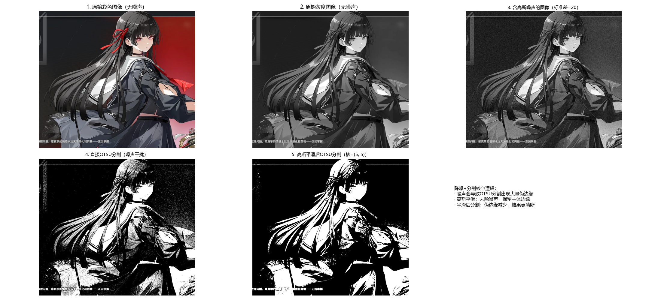
10.3.5 利用边缘信息改进全局阈值分割
核心思想:先检测边缘,再结合边缘位置调整阈值,保留边缘区域的细节。
完整代码(含效果对比)
python
# 导入必要的库
import cv2
import numpy as np
import matplotlib.pyplot as plt
import os  # 处理路径兼容性

# ===================== 核心配置项 =====================
# 替换为你自己的图片路径(绝对/相对路径均可)
IMAGE_PATH = r"../picture/LinNai.png"  # Windows示例:r"D:\images\test.png"
# Canny边缘检测参数(可调整)
CANNY_LOW = 50  # 低阈值
CANNY_HIGH = 150  # 高阈值
# 显示窗口尺寸
FIG_SIZE = (22, 10)
# ======================================================

# 设置matplotlib支持中文显示(解决标题乱码+特殊符号警告)
plt.rcParams['font.sans-serif'] = ['Microsoft YaHei', 'SimHei', 'DejaVu Sans']
plt.rcParams['axes.unicode_minus'] = False
plt.rcParams['font.family'] = 'sans-serif'


def edge_improved_threshold(img_gray, canny_low=50, canny_high=150):
    """
    边缘信息改进阈值分割
    核心原理:边缘区域保留原图灰度(保留细节),非边缘区域用OTSU阈值分割(简化背景)
    :param img_gray: 输入灰度图像
    :param canny_low: Canny边缘检测低阈值
    :param canny_high: Canny边缘检测高阈值
    :return: otsu_seg(普通OTSU分割结果), improved_seg(边缘改进分割结果)
    """
    # 步骤1:Canny边缘检测(提取图像的关键边缘)
    canny_edge = cv2.Canny(img_gray, canny_low, canny_high)

    # 步骤2:普通OTSU阈值分割(作为基础分割结果)
    _, otsu_seg = cv2.threshold(img_gray, 0, 255, cv2.THRESH_BINARY + cv2.THRESH_OTSU)

    # 步骤3:结合边缘信息改进分割
    # 逻辑:边缘区域(canny_edge>0)保留原图灰度,非边缘区域用OTSU分割结果
    improved_seg = np.where(canny_edge > 0, img_gray, otsu_seg)
    # 归一化到0-255(避免灰度值溢出,确保显示正常)
    improved_seg = np.uint8(np.clip(improved_seg, 0, 255))

    return canny_edge, otsu_seg, improved_seg


def main():
    # 1. 加载图像(优先使用自定义图片,失败则降级到内置测试图)
    # 检查路径是否存在,增加容错提示
    if not os.path.exists(IMAGE_PATH):
        print(f"警告:图片路径 {IMAGE_PATH} 不存在!")
        img_color = None
    else:
        img_color = cv2.imread(IMAGE_PATH)  # 读取彩色原图

    if img_color is None:
        print(f"自动使用内置测试图片(Lena)")
        img_color = cv2.imread(cv2.samples.findFile('lena.jpg'))

    # 转换为灰度图(分割/边缘检测要求输入灰度图)
    img_gray = cv2.cvtColor(img_color, cv2.COLOR_BGR2GRAY)

    # 2. 执行边缘改进阈值分割
    canny_edge, otsu_seg, improved_seg = edge_improved_threshold(
        img_gray,
        canny_low=CANNY_LOW,
        canny_high=CANNY_HIGH
    )

    # 3. 效果对比可视化(同一窗口展示所有结果)
    plt.figure(figsize=FIG_SIZE)

    # 子图1:原始彩色图片
    plt.subplot(2, 3, 1)
    plt.imshow(cv2.cvtColor(img_color, cv2.COLOR_BGR2RGB))
    plt.title('1. 原始彩色图像', fontsize=12)
    plt.axis('off')  # 隐藏坐标轴

    # 子图2:原始灰度图片
    plt.subplot(2, 3, 2)
    plt.imshow(img_gray, cmap='gray')
    plt.title('2. 原始灰度图像', fontsize=12)
    plt.axis('off')

    # 子图3:Canny边缘检测结果(关键中间步骤)
    plt.subplot(2, 3, 3)
    plt.imshow(canny_edge, cmap='gray')
    plt.title(f'3. Canny边缘检测(低={CANNY_LOW}, 高={CANNY_HIGH})', fontsize=11)
    plt.axis('off')

    # 子图4:普通OTSU阈值分割结果
    plt.subplot(2, 3, 4)
    plt.imshow(otsu_seg, cmap='gray')
    plt.title('4. 普通OTSU阈值分割', fontsize=11)
    plt.axis('off')

    # 子图5:边缘信息改进分割结果
    plt.subplot(2, 3, 5)
    plt.imshow(improved_seg, cmap='gray')
    plt.title('5. 边缘信息改进分割', fontsize=11)
    plt.axis('off')

    # 子图6:方法原理说明
    plt.subplot(2, 3, 6)
    plt.text(0.1, 0.8,
             '边缘改进分割核心:\n· 普通OTSU:仅黑白二值,丢失边缘细节\n· 改进策略:边缘区域保留原图灰度(细节)\n· 非边缘区域:用OTSU结果(简化背景)\n· 优势:兼顾细节保留与背景简化',
             fontsize=11, verticalalignment='top', fontfamily='sans-serif')
    plt.axis('off')
    plt.xticks([])
    plt.yticks([])

    # 调整子图间距,避免标题/图片重叠
    plt.tight_layout()
    # 显示所有子图
    plt.show()


# 程序入口
if __name__ == "__main__":
    main()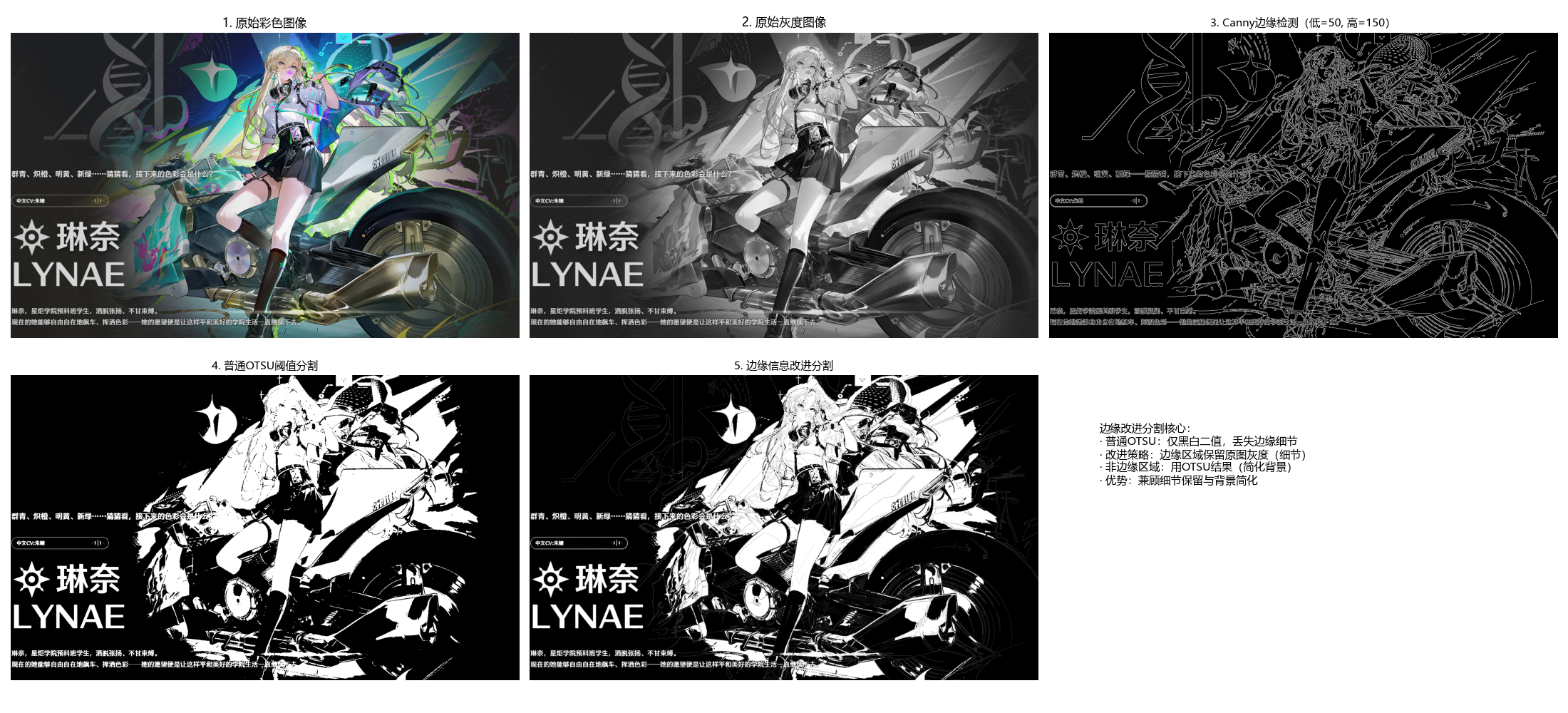
10.3.6 多阈值分割
多阈值分割将图像分为多个区域(如前景、背景、中间区域),核心是选择多个阈值 T1<T2<...<Tn。
完整代码(含效果对比)
python
# 导入必要的库
import cv2
import numpy as np
import matplotlib.pyplot as plt
import os  # 处理路径兼容性

# ===================== 核心配置项 =====================
# 替换为你自己的图片路径(绝对/相对路径均可)
IMAGE_PATH = r"../picture/Water.png"  # Windows示例:r"D:\images\test.png"
# 多阈值分割参数(可调整)
USE_AUTO_OTSU = False  # True=自动计算多类OTSU阈值,False=手动设置阈值
MANUAL_T1 = 80  # 手动阈值1(背景/中间区域分界)
MANUAL_T2 = 180  # 手动阈值2(中间/前景区域分界)
SINGLE_THRESHOLD = 127  # 单阈值分割对比用阈值
# 显示窗口尺寸
FIG_SIZE = (22, 10)
# ======================================================

# 设置matplotlib支持中文显示(解决标题乱码+特殊符号警告)
plt.rcParams['font.sans-serif'] = ['Microsoft YaHei', 'SimHei', 'DejaVu Sans']
plt.rcParams['axes.unicode_minus'] = False
plt.rcParams['font.family'] = 'sans-serif'


def multi_threshold_segmentation(img_gray, use_auto_otsu=False, manual_t1=80, manual_t2=180):
    """
    多阈值分割(三区域:背景/中间/前景)
    :param img_gray: 输入灰度图像
    :param use_auto_otsu: 是否使用多类OTSU自动计算阈值
    :param manual_t1: 手动阈值1(仅use_auto_otsu=False时生效)
    :param manual_t2: 手动阈值2(仅use_auto_otsu=False时生效)
    :return: multi_seg(多阈值分割结果), t1, t2(使用的两个阈值)
    """
    # 步骤1:确定多阈值(自动/手动)
    if use_auto_otsu:
        # 多类OTSU自动计算两个阈值(适用于三峰灰度分布图像)
        # 原理:将图像分为3类,计算使类间方差最大的两个阈值
        hist = cv2.calcHist([img_gray], [0], None, [256], [0, 256])
        hist = hist.flatten() / hist.sum()  # 归一化直方图

        max_variance = 0
        t1, t2 = 0, 0
        # 遍历所有可能的阈值组合(t1 < t2)
        for i in range(1, 255):
            for j in range(i + 1, 255):
                # 划分三类像素
                c1 = hist[:i].sum()
                c2 = hist[i:j].sum()
                c3 = hist[j:].sum()
                if c1 == 0 or c2 == 0 or c3 == 0:
                    continue
                # 计算各类均值
                m1 = (hist[:i] * np.arange(i)).sum() / c1
                m2 = (hist[i:j] * np.arange(i, j)).sum() / c2
                m3 = (hist[j:] * np.arange(j, 256)).sum() / c3
                # 全局均值
                m = c1 * m1 + c2 * m2 + c3 * m3
                # 类间方差
                variance = c1 * (m1 - m) ** 2 + c2 * (m2 - m) ** 2 + c3 * (m3 - m) ** 2
                if variance > max_variance:
                    max_variance = variance
                    t1, t2 = i, j
    else:
        # 使用手动设置的阈值
        t1, t2 = manual_t1, manual_t2

    # 步骤2:多阈值分割(三区域)
    multi_seg = np.zeros_like(img_gray, dtype=np.uint8)
    multi_seg[img_gray < t1] = 0  # 背景(黑色)
    multi_seg[(img_gray >= t1) & (img_gray < t2)] = 128  # 中间区域(灰色)
    multi_seg[img_gray >= t2] = 255  # 前景(白色)

    return multi_seg, t1, t2


def main():
    # 1. 加载图像(优先使用自定义图片,失败则降级到内置测试图)
    # 检查路径是否存在,增加容错提示
    if not os.path.exists(IMAGE_PATH):
        print(f"警告:图片路径 {IMAGE_PATH} 不存在!")
        img_color = None
    else:
        img_color = cv2.imread(IMAGE_PATH)  # 读取彩色原图

    if img_color is None:
        print(f"自动使用内置测试图片(Lena)")
        img_color = cv2.imread(cv2.samples.findFile('lena.jpg'))

    # 转换为灰度图(阈值分割要求输入灰度图)
    img_gray = cv2.cvtColor(img_color, cv2.COLOR_BGR2GRAY)

    # 2. 执行阈值分割
    # 多阈值分割
    multi_seg, t1, t2 = multi_threshold_segmentation(
        img_gray,
        use_auto_otsu=USE_AUTO_OTSU,
        manual_t1=MANUAL_T1,
        manual_t2=MANUAL_T2
    )
    # 单阈值分割(对比组)
    _, single_seg = cv2.threshold(img_gray, SINGLE_THRESHOLD, 255, cv2.THRESH_BINARY)

    # 3. 效果对比可视化(同一窗口展示所有结果)
    plt.figure(figsize=FIG_SIZE)

    # 子图1:原始彩色图片
    plt.subplot(2, 3, 1)
    plt.imshow(cv2.cvtColor(img_color, cv2.COLOR_BGR2RGB))
    plt.title('1. 原始彩色图像', fontsize=12)
    plt.axis('off')  # 隐藏坐标轴

    # 子图2:原始灰度图片
    plt.subplot(2, 3, 2)
    plt.imshow(img_gray, cmap='gray')
    plt.title('2. 原始灰度图像', fontsize=12)
    plt.axis('off')

    # 子图3:单阈值分割结果(二值)
    plt.subplot(2, 3, 3)
    plt.imshow(single_seg, cmap='gray')
    plt.title(f'3. 单阈值分割(阈值={SINGLE_THRESHOLD})', fontsize=11)
    plt.axis('off')

    # 子图4:多阈值分割结果(三区域)
    plt.subplot(2, 3, 4)
    plt.imshow(multi_seg, cmap='gray')
    threshold_type = "自动OTSU" if USE_AUTO_OTSU else "手动"
    plt.title(f'4. 多阈值分割({threshold_type},T1={t1}, T2={t2})', fontsize=11)
    plt.axis('off')

    # 子图5:灰度直方图+阈值标记
    plt.subplot(2, 3, 5)
    # 计算灰度直方图
    hist = cv2.calcHist([img_gray], [0], None, [256], [0, 256])
    plt.plot(hist, color='black', label='灰度直方图')
    # 标记单阈值(红色虚线)
    plt.axvline(x=SINGLE_THRESHOLD, color='red', linestyle='--', label=f'单阈值={SINGLE_THRESHOLD}')
    # 标记多阈值(绿色/蓝色实线)
    plt.axvline(x=t1, color='green', linestyle='-', label=f'多阈值T1={t1}')
    plt.axvline(x=t2, color='blue', linestyle='-', label=f'多阈值T2={t2}')
    plt.xlim([0, 255])
    plt.xlabel('灰度值')
    plt.ylabel('像素数量')
    plt.title('5. 灰度直方图+阈值标记', fontsize=11)
    plt.legend(fontsize=9)

    # 子图6:方法对比说明
    plt.subplot(2, 3, 6)
    plt.text(0.1, 0.8,
             '单阈值vs多阈值分割:\n· 单阈值:仅分前景/背景(丢失中间细节)\n· 多阈值:分背景/中间/前景(保留更多层次)\n· 适用场景:多阈值适配三峰灰度分布图像\n(如人像:背景/皮肤/头发)',
             fontsize=11, verticalalignment='top', fontfamily='sans-serif')
    plt.axis('off')
    plt.xticks([])
    plt.yticks([])

    # 调整子图间距,避免标题/图片重叠
    plt.tight_layout()
    # 显示所有子图
    plt.show()


# 程序入口
if __name__ == "__main__":
    main()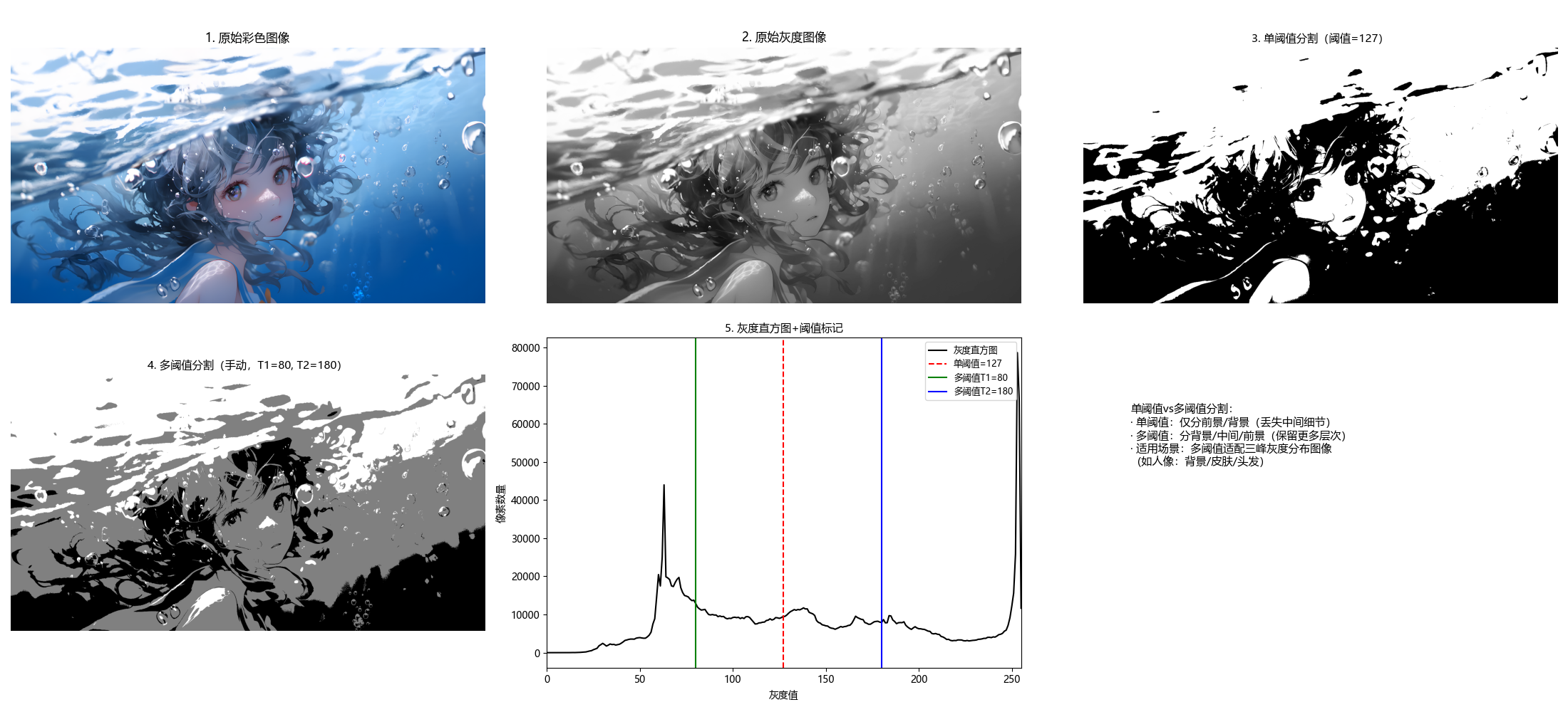
10.3.7 可变阈值分割
可变阈值(局部阈值):图像不同区域使用不同的阈值,适用于光照不均匀的图像。
完整代码(含效果对比)
python
# 导入必要的库
import cv2
import numpy as np
import matplotlib.pyplot as plt
import os  # 处理路径兼容性

# ===================== 核心配置项 =====================
# 替换为你自己的图片路径(绝对/相对路径均可)
IMAGE_PATH = r"../picture/TianHuoSanXuanBian.jpg"  # Windows示例:r"D:\images\test.png"
# 自适应阈值分割参数(可调整)
ADAPTIVE_METHOD = cv2.ADAPTIVE_THRESH_GAUSSIAN_C  # 高斯加权均值(可选:ADAPTIVE_THRESH_MEAN_C=简单均值)
BLOCK_SIZE = 11  # 邻域大小(奇数,越大覆盖范围越广)
C_VALUE = 2  # 常数(阈值=邻域均值 - C,可正可负)
# 光照不均匀模拟参数
LIGHT_GRADIENT = 100  # 光照梯度强度(越大光照不均越明显)
# 显示窗口尺寸
FIG_SIZE = (22, 10)
# ======================================================

# 设置matplotlib支持中文显示(解决标题乱码+特殊符号警告)
plt.rcParams['font.sans-serif'] = ['Microsoft YaHei', 'SimHei', 'DejaVu Sans']
plt.rcParams['axes.unicode_minus'] = False
plt.rcParams['font.family'] = 'sans-serif'


def adaptive_threshold_segmentation(img_gray, adaptive_method=cv2.ADAPTIVE_THRESH_GAUSSIAN_C, block_size=11, c=2):
    """
    自适应(可变)阈值分割
    核心原理:对每个像素,用其邻域的均值(/高斯加权均值)减去常数作为阈值,适配局部光照变化
    :param img_gray: 输入灰度图像(通常是光照不均匀的图)
    :param adaptive_method: 自适应方法(GAUSSIAN_C/MEAN_C)
    :param block_size: 邻域大小(奇数,如11、15、21)
    :param c: 常数(阈值 = 邻域均值 - c)
    :return: adaptive_seg(自适应阈值分割结果)
    """
    # 自适应阈值分割(解决全局阈值在光照不均场景下的失效问题)
    adaptive_seg = cv2.adaptiveThreshold(
        img_gray,  # 输入灰度图
        255,  # 最大值(超过阈值设为255)
        adaptive_method,  # 邻域均值计算方式
        cv2.THRESH_BINARY,  # 二值化模式
        block_size,  # 邻域大小(奇数)
        c  # 常数(调整阈值偏移)
    )
    return adaptive_seg


def add_light_gradient(img_gray, gradient_strength=100):
    """
    为灰度图像添加水平光照梯度(模拟光照不均匀场景)
    :param img_gray: 输入灰度图像
    :param gradient_strength: 光照梯度强度(0-100,越大不均越明显)
    :return: 光照不均匀的灰度图像
    """
    rows, cols = img_gray.shape
    # 生成水平光照梯度(从左到右亮度递增)
    light = np.linspace(0, gradient_strength, cols).astype(np.float32)
    light = np.tile(light, (rows, 1))  # 扩展到与原图同尺寸
    # 叠加光照(避免像素值溢出0-255)
    img_with_light = img_gray.astype(np.float32) + light
    img_with_light = np.clip(img_with_light, 0, 255).astype(np.uint8)
    return img_with_light


def main():
    # 1. 加载图像(优先使用自定义图片,失败则降级到内置测试图)
    # 检查路径是否存在,增加容错提示
    if not os.path.exists(IMAGE_PATH):
        print(f"警告:图片路径 {IMAGE_PATH} 不存在!")
        img_color = None
    else:
        img_color = cv2.imread(IMAGE_PATH)  # 读取彩色原图

    if img_color is None:
        print(f"自动使用内置测试图片(Lena)")
        img_color = cv2.imread(cv2.samples.findFile('lena.jpg'))

    # 转换为灰度图(阈值分割要求输入灰度图)
    img_gray_original = cv2.cvtColor(img_color, cv2.COLOR_BGR2GRAY)

    # 2. 模拟光照不均匀场景(核心测试条件)
    img_gray_uneven = add_light_gradient(img_gray_original, gradient_strength=LIGHT_GRADIENT)

    # 3. 执行阈值分割
    # 自适应阈值分割(改进组)
    adaptive_seg = adaptive_threshold_segmentation(
        img_gray_uneven,
        adaptive_method=ADAPTIVE_METHOD,
        block_size=BLOCK_SIZE,
        c=C_VALUE
    )
    # 全局OTSU分割(对比组,展示光照不均下的失效)
    _, global_seg = cv2.threshold(img_gray_uneven, 0, 255, cv2.THRESH_BINARY + cv2.THRESH_OTSU)

    # 4. 效果对比可视化(同一窗口展示所有结果)
    plt.figure(figsize=FIG_SIZE)

    # 子图1:原始彩色图像(无光照不均)
    plt.subplot(2, 3, 1)
    plt.imshow(cv2.cvtColor(img_color, cv2.COLOR_BGR2RGB))
    plt.title('1. 原始彩色图像(无光照不均)', fontsize=12)
    plt.axis('off')  # 隐藏坐标轴

    # 子图2:原始灰度图像(无光照不均)
    plt.subplot(2, 3, 2)
    plt.imshow(img_gray_original, cmap='gray')
    plt.title('2. 原始灰度图像(无光照不均)', fontsize=12)
    plt.axis('off')

    # 子图3:光照不均匀的灰度图像
    plt.subplot(2, 3, 3)
    plt.imshow(img_gray_uneven, cmap='gray')
    plt.title(f'3. 光照不均匀的灰度图像(梯度={LIGHT_GRADIENT})', fontsize=11)
    plt.axis('off')

    # 子图4:全局OTSU分割结果(效果差)
    plt.subplot(2, 3, 4)
    plt.imshow(global_seg, cmap='gray')
    plt.title('4. 全局OTSU分割(光照不均失效)', fontsize=11)
    plt.axis('off')

    # 子图5:自适应阈值分割结果(效果好)
    plt.subplot(2, 3, 5)
    plt.imshow(adaptive_seg, cmap='gray')
    method_name = "高斯加权均值" if ADAPTIVE_METHOD == cv2.ADAPTIVE_THRESH_GAUSSIAN_C else "简单均值"
    plt.title(f'5. 自适应阈值分割({method_name},块={BLOCK_SIZE})', fontsize=11)
    plt.axis('off')

    # 子图6:方法原理说明
    plt.subplot(2, 3, 6)
    plt.text(0.1, 0.8,
             '自适应阈值核心优势:\n· 全局阈值:整图用一个阈值,光照不均时失效\n· 自适应阈值:每个像素用「邻域均值-C」做阈值\n· 适配局部光照变化,解决全局阈值的局限性\n· 高斯加权:邻域中心像素权重更高,效果更优',
             fontsize=11, verticalalignment='top', fontfamily='sans-serif')
    plt.axis('off')
    plt.xticks([])
    plt.yticks([])

    # 调整子图间距,避免标题/图片重叠
    plt.tight_layout()
    # 显示所有子图
    plt.show()


# 程序入口
if __name__ == "__main__":
    main()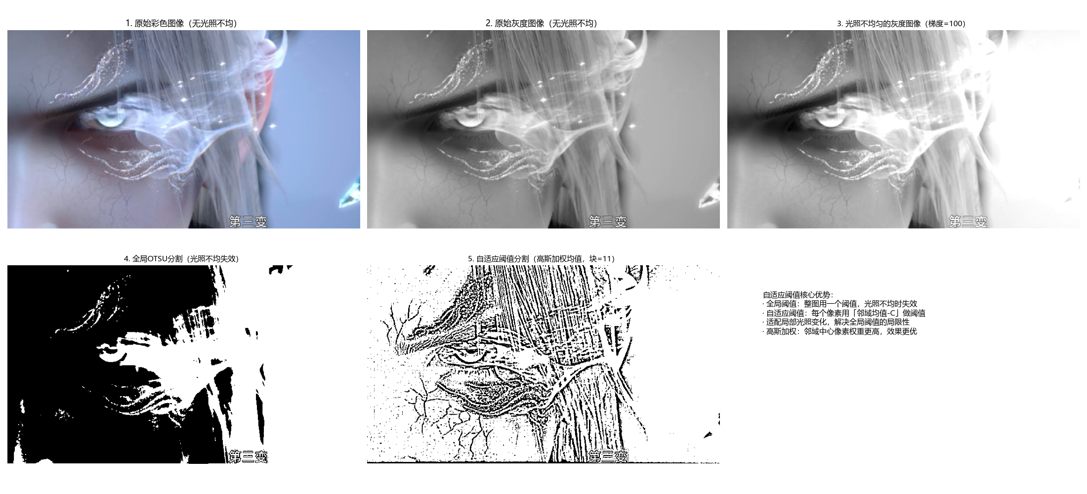
10.3.8 多变量阈值分割
多变量阈值:基于多个特征(如 RGB 三通道、灰度 + 梯度)进行阈值分割,适用于彩色图像。
完整代码(含效果对比)
python
# 导入必要的库
import cv2
import numpy as np
import matplotlib.pyplot as plt
import os  # 处理路径兼容性

# ===================== 核心配置项 =====================
# 替换为你自己的彩色图片路径(绝对/相对路径均可)
IMAGE_PATH = r"../picture/KaTiXiYa.png"  # Windows示例:r"D:\images\color_test.png"
# 多变量(RGB)阈值配置(可独立调整每个通道的阈值)
R_THRESH = 100  # R通道阈值
G_THRESH = 100  # G通道阈值
B_THRESH = 100  # B通道阈值
# 单通道灰度分割阈值
GRAY_THRESH = 127
# 显示窗口尺寸
FIG_SIZE = (22, 12)
# ======================================================

# 设置matplotlib支持中文显示(解决标题乱码+特殊符号警告)
plt.rcParams['font.sans-serif'] = ['Microsoft YaHei', 'SimHei', 'DejaVu Sans']
plt.rcParams['axes.unicode_minus'] = False
plt.rcParams['font.family'] = 'sans-serif'


def multi_variable_threshold(img_bgr, r_thresh=100, g_thresh=100, b_thresh=100):
    """
    多变量阈值分割(彩色图像,RGB三通道)
    核心原理:基于RGB三个通道的灰度值联合判断,而非单通道灰度,能更精准分割彩色目标
    :param img_bgr: 输入BGR彩色图像(cv2默认读取格式)
    :param r_thresh: R通道阈值
    :param g_thresh: G通道阈值
    :param b_thresh: B通道阈值
    :return: seg(多变量分割结果,二值图), r, g, b(分离后的RGB通道)
    """
    # 步骤1:将BGR转为RGB(匹配视觉认知的通道顺序)
    img_rgb = cv2.cvtColor(img_bgr, cv2.COLOR_BGR2RGB)
    # 步骤2:分离RGB三个通道
    r, g, b = cv2.split(img_rgb)

    # 步骤3:多变量阈值判断
    # 逻辑:同时满足R>r_thresh、G>g_thresh、B>b_thresh的像素为前景(255),否则为背景(0)
    # 可根据需求修改逻辑(如:R<50且G>150且B<50 分割绿色目标)
    seg = np.zeros_like(r, dtype=np.uint8)
    seg[(r > r_thresh) & (g > g_thresh) & (b > b_thresh)] = 255

    return seg, r, g, b


def main():
    # 1. 加载彩色图像(优先使用自定义图片,失败则降级到内置测试图)
    # 检查路径是否存在,增加容错提示
    if not os.path.exists(IMAGE_PATH):
        print(f"警告:图片路径 {IMAGE_PATH} 不存在!")
        img_bgr = None
    else:
        img_bgr = cv2.imread(IMAGE_PATH)  # cv2默认读取为BGR格式

    if img_bgr is None:
        print(f"自动使用内置测试图片(Lena彩色图)")
        img_bgr = cv2.imread(cv2.samples.findFile('lena.jpg'))

    # 转为RGB格式(用于matplotlib显示)
    img_rgb = cv2.cvtColor(img_bgr, cv2.COLOR_BGR2RGB)

    # 2. 执行阈值分割
    # 多变量(RGB)阈值分割
    multi_var_seg, r_channel, g_channel, b_channel = multi_variable_threshold(
        img_bgr,
        r_thresh=R_THRESH,
        g_thresh=G_THRESH,
        b_thresh=B_THRESH
    )
    # 单通道(灰度)阈值分割(对比组)
    gray = cv2.cvtColor(img_bgr, cv2.COLOR_BGR2GRAY)
    _, gray_seg = cv2.threshold(gray, GRAY_THRESH, 255, cv2.THRESH_BINARY)

    # 3. 效果对比可视化(同一窗口展示所有结果)
    plt.figure(figsize=FIG_SIZE)

    # 子图1:原始彩色图像(RGB)
    plt.subplot(3, 3, 1)
    plt.imshow(img_rgb)
    plt.title('1. 原始彩色图像(RGB)', fontsize=12)
    plt.axis('off')

    # 子图2:单通道灰度图
    plt.subplot(3, 3, 2)
    plt.imshow(gray, cmap='gray')
    plt.title('2. 单通道灰度图', fontsize=12)
    plt.axis('off')

    # 子图3:单通道灰度阈值分割结果
    plt.subplot(3, 3, 3)
    plt.imshow(gray_seg, cmap='gray')
    plt.title(f'3. 灰度阈值分割(阈值={GRAY_THRESH})', fontsize=11)
    plt.axis('off')

    # 子图4-6:RGB三个通道的灰度分布
    plt.subplot(3, 3, 4)
    plt.imshow(r_channel, cmap='gray')
    plt.title(f'4. R通道(阈值={R_THRESH})', fontsize=11)
    plt.axis('off')

    plt.subplot(3, 3, 5)
    plt.imshow(g_channel, cmap='gray')
    plt.title(f'5. G通道(阈值={G_THRESH})', fontsize=11)
    plt.axis('off')

    plt.subplot(3, 3, 6)
    plt.imshow(b_channel, cmap='gray')
    plt.title(f'6. B通道(阈值={B_THRESH})', fontsize=11)
    plt.axis('off')

    # 子图7:多变量(RGB)阈值分割结果
    plt.subplot(3, 3, 7)
    plt.imshow(multi_var_seg, cmap='gray')
    plt.title(f'7. RGB多变量阈值分割(R>{R_THRESH}, G>{G_THRESH}, B>{B_THRESH})', fontsize=11)
    plt.axis('off')

    # 子图8:多变量分割逻辑说明
    plt.subplot(3, 3, 8)
    plt.text(0.1, 0.8,
             '多变量分割优势:\n· 单通道灰度:丢失彩色信息,分割精度低\n· RGB多变量:利用色彩信息精准分割\n· 可自定义逻辑:如分割红色(R>200, G<50, B<50)\n· 适配彩色目标分割场景',
             fontsize=10, verticalalignment='top', fontfamily='sans-serif')
    plt.axis('off')
    plt.xticks([])
    plt.yticks([])

    # 隐藏最后一个子图(布局美观)
    plt.subplot(3, 3, 9)
    plt.axis('off')

    # 调整子图间距,避免标题/图片重叠
    plt.tight_layout()
    # 显示所有子图
    plt.show()


# 程序入口
if __name__ == "__main__":
    main()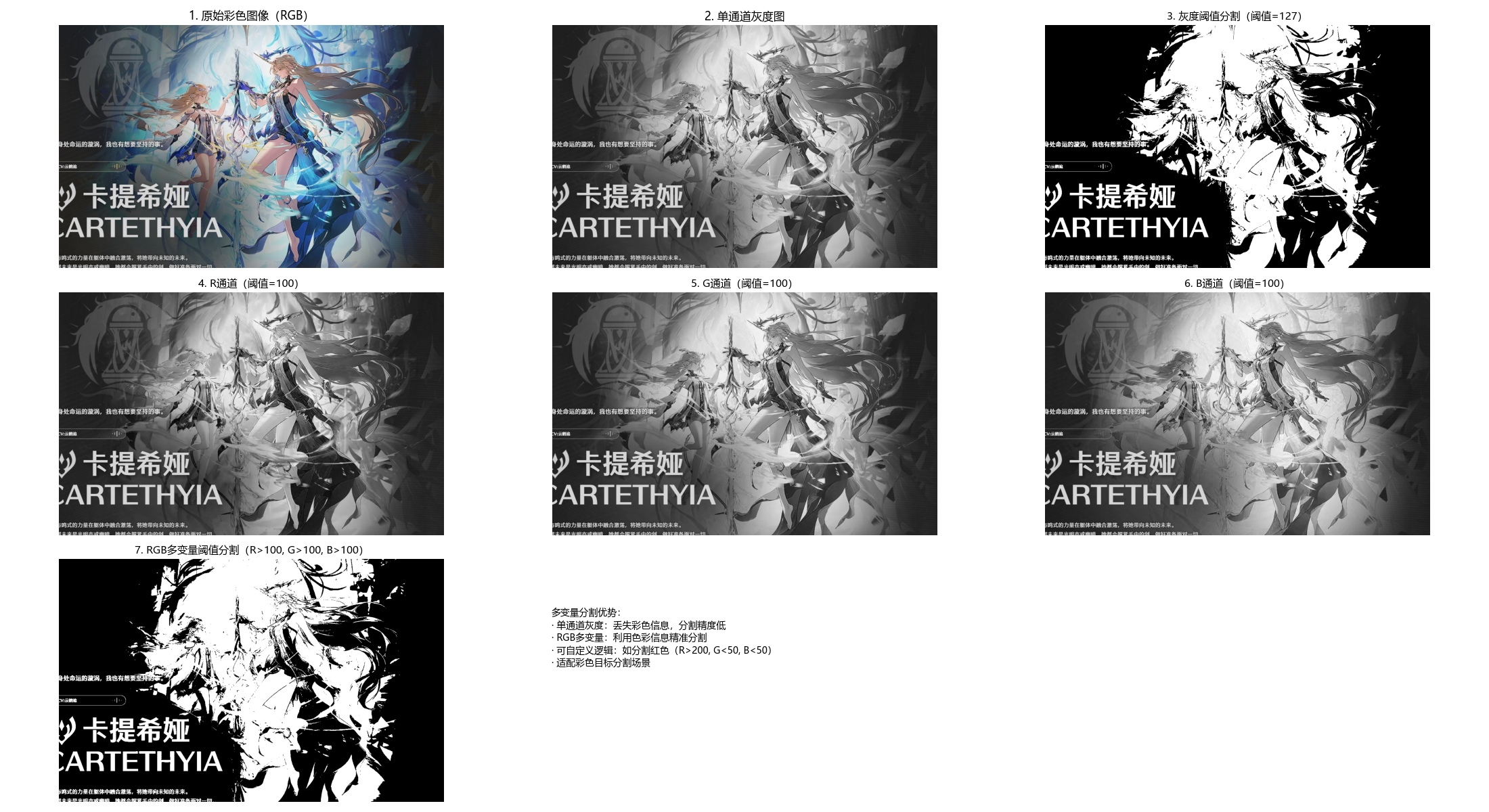
10.4 基于区域的分割
10.4.1 区域生长
原理
区域生长是从种子点开始,将相邻且满足相似性准则(如灰度差小于阈值)的像素合并到种子区域的过程,核心步骤:
- 选择种子点;
- 遍历种子点邻域像素,判断是否满足相似性准则;
- 合并满足条件的像素,作为新的种子点;
- 重复步骤 2-3,直到无新像素可合并。
完整代码(含效果对比)
python
# 导入必要的库
import cv2
import numpy as np
import matplotlib.pyplot as plt
import os
from collections import deque  # 高效队列,替代列表pop(0)
import matplotlib.cm as cm

# ===================== 核心配置项 =====================
# 替换为你自己的图片路径(绝对/相对路径均可)
IMAGE_PATH = r"../picture/XiaoYan.jpg"  # Windows示例:r"D:\images\test.png"
# 区域生长参数配置
SEED_X = 256  # 种子点X坐标(列)
SEED_Y = 256  # 种子点Y坐标(行)
GROWTH_THRESHOLD = 15  # 灰度差阈值(越小生长区域越精细,越大范围越广)
USE_MOUSE_SEED = False  # True=鼠标点击选种子点,False=使用配置的种子点
# 显示窗口尺寸
FIG_SIZE = (22, 10)
# ======================================================

# 设置matplotlib支持中文显示(解决标题乱码+特殊符号警告)
plt.rcParams['font.sans-serif'] = ['Microsoft YaHei', 'SimHei', 'DejaVu Sans']
plt.rcParams['axes.unicode_minus'] = False
plt.rcParams['font.family'] = 'sans-serif'


def region_growing(img_gray, seed, threshold=10):
    """
    区域生长分割(8邻域)
    核心原理:从种子点出发,将灰度差小于阈值的邻域像素纳入同一区域,逐步生长
    :param img_gray: 输入灰度图像
    :param seed: 种子点坐标 (x,y) → (列,行)
    :param threshold: 灰度差阈值(0-255)
    :return: seg(区域生长结果,二值图), seed_val(种子点灰度值)
    """
    rows, cols = img_gray.shape
    # 初始化分割结果(0=背景,255=生长区域)
    seg = np.zeros_like(img_gray, dtype=np.uint8)
    # 检查种子点是否在图像范围内
    if not (0 <= seed[0] < cols and 0 <= seed[1] < rows):
        print(f"警告:种子点({seed[0]},{seed[1]})超出图像范围,自动调整到中心")
        seed = (cols // 2, rows // 2)

    # 关键修复:将种子点灰度值转为int32,避免uint8溢出
    seed_val = int(img_gray[seed[1], seed[0]])
    # 关键修复:将图像转为int32,避免减法溢出
    img_int = img_gray.astype(np.int32)

    # 待处理像素队列(用deque提升效率)
    queue = deque([seed])
    # 标记已处理像素(避免重复处理)
    processed = np.zeros_like(img_gray, dtype=bool)
    processed[seed[1], seed[0]] = True

    # 8邻域方向(上下左右+四个对角线)
    directions = [(-1, -1), (-1, 0), (-1, 1),
                  (0, -1), (0, 1),
                  (1, -1), (1, 0), (1, 1)]

    # 区域生长核心循环
    while queue:
        x, y = queue.popleft()  # 取出队列头部像素
        seg[y, x] = 255  # 标记为生长区域

        # 遍历8邻域像素
        for dx, dy in directions:
            nx = x + dx  # 邻域像素X坐标
            ny = y + dy  # 邻域像素Y坐标
            # 检查:1.坐标在图像内 2.未处理过
            if 0 <= nx < cols and 0 <= ny < rows and not processed[ny, nx]:
                # 关键修复:使用int32类型计算灰度差,避免溢出
                gray_diff = abs(img_int[ny, nx] - seed_val)
                if gray_diff < threshold:
                    processed[ny, nx] = True
                    queue.append((nx, ny))

    return seg, seed_val


def mouse_select_seed(event, x, y, flags, param):
    """
    鼠标点击选择种子点的回调函数
    """
    global selected_seed
    if event == cv2.EVENT_LBUTTONDOWN:
        selected_seed = (x, y)
        print(f"已选择种子点:(X={x}, Y={y}),灰度值={int(param[y, x])}")  # 转为int避免显示异常
        # 标记种子点并显示
        img_mark = cv2.cvtColor(param, cv2.COLOR_GRAY2BGR)
        cv2.circle(img_mark, (x, y), 5, (0, 0, 255), -1)
        cv2.imshow("选择种子点(点击后关闭窗口)", img_mark)


def main():
    global selected_seed
    selected_seed = None

    # 1. 加载灰度图像(优先使用自定义图片,失败则降级到内置测试图)
    if not os.path.exists(IMAGE_PATH):
        print(f"警告:图片路径 {IMAGE_PATH} 不存在!")
        img_gray = None
    else:
        img_gray = cv2.imread(IMAGE_PATH, 0)  # 直接读取为灰度图

    if img_gray is None:
        print(f"自动使用内置测试图片(Lena灰度图)")
        img_gray = cv2.imread(cv2.samples.findFile('lena.jpg'), 0)

    rows, cols = img_gray.shape
    # 默认种子点(中心位置)
    default_seed = (SEED_X, SEED_Y) if (0 <= SEED_X < cols and 0 <= SEED_Y < rows) else (cols // 2, rows // 2)

    # 2. 选择种子点(交互/默认)
    if USE_MOUSE_SEED:
        cv2.namedWindow("选择种子点(点击后关闭窗口)")
        cv2.setMouseCallback("选择种子点(点击后关闭窗口)", mouse_select_seed, img_gray)
        cv2.imshow("选择种子点(点击后关闭窗口)", img_gray)
        cv2.waitKey(0)
        cv2.destroyAllWindows()
        seed = selected_seed if selected_seed is not None else default_seed
    else:
        seed = default_seed
        print(f"使用默认种子点:(X={seed[0]}, Y={seed[1]}),灰度值={int(img_gray[seed[1], seed[0]])}")

    # 3. 执行区域生长分割
    rg_seg, seed_val = region_growing(img_gray, seed, threshold=GROWTH_THRESHOLD)

    # 4. 生成灰度差热力图(辅助理解生长逻辑)
    gray_diff = np.abs(img_gray.astype(np.int32) - seed_val).astype(np.float32)  # 修复溢出
    gray_diff_norm = gray_diff / GROWTH_THRESHOLD  # 归一化到阈值范围
    gray_diff_norm = np.clip(gray_diff_norm, 0, 1)  # 超过阈值的设为1

    # 5. 效果对比可视化(同一窗口展示所有结果)
    plt.figure(figsize=FIG_SIZE)

    # 子图1:原始图像+种子点标记
    plt.subplot(2, 3, 1)
    plt.imshow(img_gray, cmap='gray')
    plt.scatter(seed[0], seed[1], color='red', s=80, marker='*')  # 红色星号标记种子点
    plt.title(f'1. 原始图像(种子点灰度={seed_val})', fontsize=12)
    plt.axis('off')

    # 子图2:灰度差热力图(与种子点的灰度差)
    plt.subplot(2, 3, 2)
    im = plt.imshow(gray_diff_norm, cmap=cm.jet)
    plt.colorbar(im, shrink=0.8, label='灰度差/阈值')
    plt.axhline(y=seed[1], color='white', linestyle='--', alpha=0.5)
    plt.axvline(x=seed[0], color='white', linestyle='--', alpha=0.5)
    plt.title(f'2. 灰度差热力图(阈值={GROWTH_THRESHOLD})', fontsize=11)
    plt.axis('off')

    # 子图3:区域生长分割结果(二值图)
    plt.subplot(2, 3, 3)
    plt.imshow(rg_seg, cmap='gray')
    plt.title('3. 区域生长分割结果', fontsize=11)
    plt.axis('off')

    # 子图4:分割结果叠加原图(绿色标记生长区域)
    overlay = cv2.cvtColor(img_gray, cv2.COLOR_GRAY2BGR)
    overlay[rg_seg == 255] = [0, 255, 0]  # 生长区域标为绿色
    plt.subplot(2, 3, 4)
    plt.imshow(cv2.cvtColor(overlay, cv2.COLOR_BGR2RGB))
    plt.title('4. 分割结果叠加原图(绿色)', fontsize=11)
    plt.axis('off')

    # 子图5:生长区域的灰度分布
    plt.subplot(2, 3, 5)
    growth_gray = img_gray[rg_seg == 255]
    plt.hist(growth_gray, bins=50, color='green', alpha=0.7)
    plt.axvline(x=seed_val, color='red', linestyle='--', label=f'种子点灰度={seed_val}')
    plt.axvline(x=seed_val + GROWTH_THRESHOLD, color='orange', linestyle='--',
                label=f'上限={seed_val + GROWTH_THRESHOLD}')
    plt.axvline(x=seed_val - GROWTH_THRESHOLD, color='orange', linestyle='--',
                label=f'下限={seed_val - GROWTH_THRESHOLD}')
    plt.xlabel('灰度值')
    plt.ylabel('像素数量')
    plt.title('5. 生长区域灰度分布', fontsize=11)
    plt.legend(fontsize=9)

    # 子图6:方法原理说明
    plt.subplot(2, 3, 6)
    plt.text(0.1, 0.8,
             '区域生长核心逻辑:\n· 从种子点出发,8邻域逐步扩展\n· 仅纳入灰度差<阈值的像素\n· 阈值越小:区域越精细,范围越小\n· 阈值越大:区域越宽泛,易包含噪声',
             fontsize=11, verticalalignment='top', fontfamily='sans-serif')
    plt.axis('off')
    plt.xticks([])
    plt.yticks([])

    # 调整子图间距
    plt.tight_layout()
    plt.show()


# 程序入口
if __name__ == "__main__":
    main()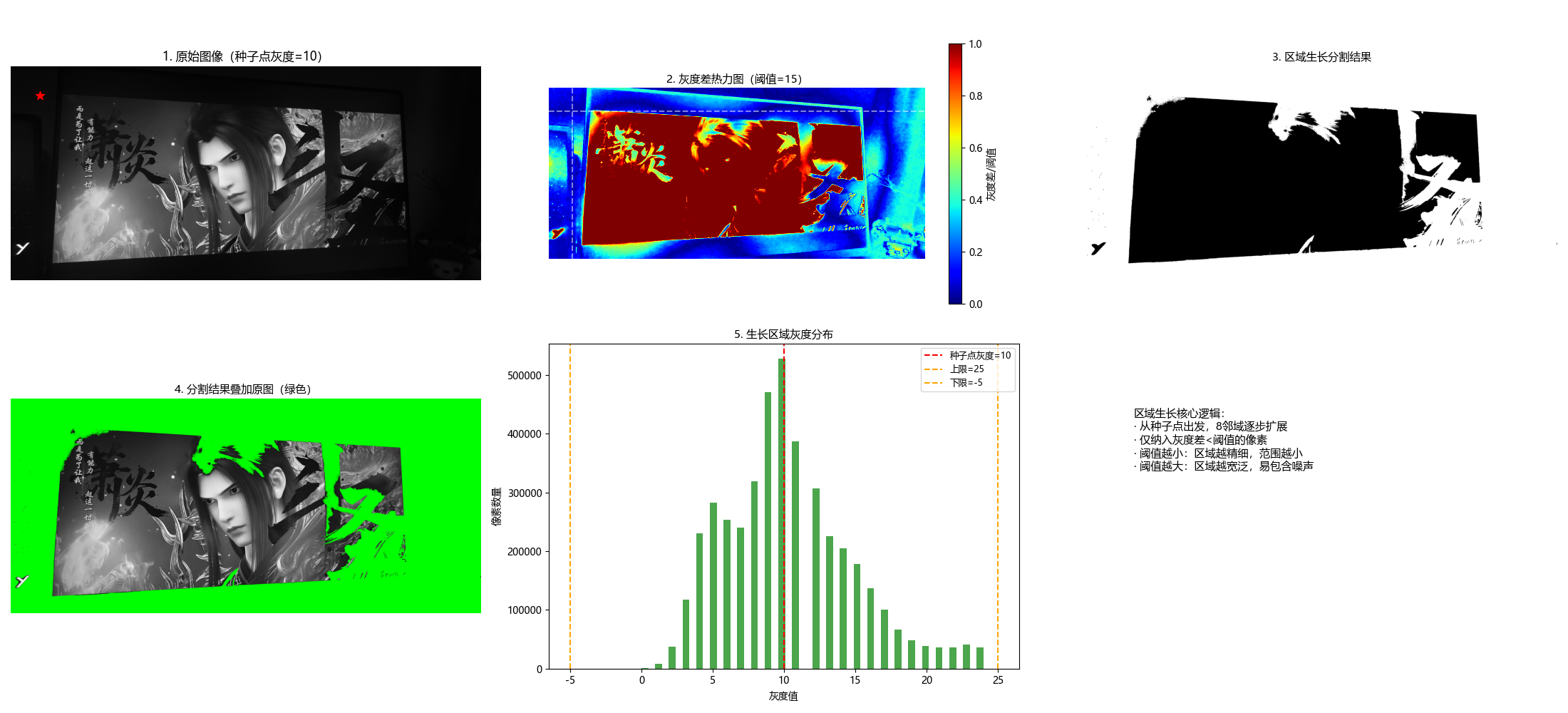
10.4.2 区域分裂与合并
原理
区域分裂与合并是 "先分裂、后合并" 的分割方法:
- 分裂:将图像递归划分为 4 个子块,若子块内像素不满足一致性准则,则继续分裂;
- 合并:对相邻的子块,若合并后满足一致性准则,则合并为一个大区域。
完整代码(含效果对比)
python
# 导入必要的库
import cv2
import numpy as np
import matplotlib.pyplot as plt
import os

# ===================== 核心配置项 =====================
# 替换为你自己的图片路径
IMAGE_PATH = r"../picture/AALi.jpg"  # Windows示例:r"D:\images\test.png"
# 分裂阈值(方差越小,分裂越细,分割越精细)
SPLIT_THRESHOLD = 20
# 合并阈值(均值差越小,合并越严格)
MERGE_THRESHOLD = 10
# 最小块尺寸(防止过度分裂)
MIN_BLOCK_SIZE = 4
# 显示窗口尺寸
FIG_SIZE = (22, 12)
# ======================================================

# 设置matplotlib支持中文显示
plt.rcParams['font.sans-serif'] = ['Microsoft YaHei', 'SimHei', 'DejaVu Sans']
plt.rcParams['axes.unicode_minus'] = False
plt.rcParams['font.family'] = 'sans-serif'


def split_and_merge(img_gray, split_threshold=20, merge_threshold=10, min_block_size=4):
    """
    区域分裂与合并(改进版)
    核心原理:
    1. 分裂:将图像递归分裂为4个子块,直到块内灰度方差<阈值或达到最小尺寸
    2. 合并:相邻且灰度均值差<阈值的块合并为同一区域
    :param img_gray: 输入灰度图像
    :param split_threshold: 分裂阈值(灰度方差)
    :param merge_threshold: 合并阈值(均值差)
    :param min_block_size: 最小块尺寸
    :return: seg(分割结果), blocks_info(块信息,用于可视化)
    """
    rows, cols = img_gray.shape

    # 步骤1:补全图像尺寸为2的幂次(方便递归分裂)
    def pad_to_power2(img):
        h, w = img.shape
        new_h = 1
        while new_h < h:
            new_h *= 2
        new_w = 1
        while new_w < w:
            new_w *= 2
        pad_h = new_h - h
        pad_w = new_w - w
        # 填充(只在右侧和下侧填充,避免影响左侧/上侧的原始图像)
        padded = cv2.copyMakeBorder(img, 0, pad_h, 0, pad_w,
                                    cv2.BORDER_REPLICATE, value=0)  # 复制边缘填充,更自然
        return padded, (h, w)

    img_padded, (orig_h, orig_w) = pad_to_power2(img_gray)
    h, w = img_padded.shape
    blocks_info = []  # 存储块信息:(x, y, w, h, mean, var)

    # 步骤2:递归分裂函数
    def split(block, x, y, block_w, block_h):
        """
        递归分裂块
        :param block: 当前块图像
        :param x, y: 块在原图中的左上角坐标
        :param block_w, block_h: 块的宽高
        """
        # 计算块的灰度均值和方差
        mean_val = np.mean(block)
        var_val = np.var(block)

        # 终止条件:达到最小尺寸 或 方差小于阈值(块内一致性好)
        if block_w <= min_block_size or block_h <= min_block_size or var_val < split_threshold:
            blocks_info.append((x, y, block_w, block_h, mean_val, var_val))
            return

        # 分裂为4个子块
        h2, w2 = block_h // 2, block_w // 2
        # 左上
        split(block[:h2, :w2], x, y, w2, h2)
        # 右上
        split(block[:h2, w2:], x + w2, y, w2, h2)
        # 左下
        split(block[h2:, :w2], x, y + h2, w2, h2)
        # 右下
        split(block[h2:, w2:], x + w2, y + h2, w2, h2)

    # 执行分裂(从整个图像开始)
    split(img_padded, 0, 0, w, h)

    # 步骤3:合并相似块(改进版:相邻块合并)
    seg = np.zeros_like(img_padded)
    merged = np.zeros(len(blocks_info), dtype=bool)  # 标记是否已合并

    # 遍历所有块,尝试合并相邻块
    for i in range(len(blocks_info)):
        if merged[i]:
            continue
        x1, y1, w1, h1, mean1, var1 = blocks_info[i]

        # 查找相邻块(右侧和下侧,避免重复合并)
        for j in range(i + 1, len(blocks_info)):
            if merged[j]:
                continue
            x2, y2, w2, h2, mean2, var2 = blocks_info[j]

            # 判断是否相邻
            is_adjacent = False
            # 右侧相邻
            if (x2 == x1 + w1) and (y2 == y1) and (h2 == h1):
                is_adjacent = True
            # 下侧相邻
            elif (y2 == y1 + h1) and (x2 == x1) and (w2 == w1):
                is_adjacent = True

            # 相邻且均值差小于合并阈值,则合并
            if is_adjacent and abs(mean1 - mean2) < merge_threshold:
                # 标记为已合并
                merged[j] = True
                # 扩展当前块的范围
                x1 = min(x1, x2)
                y1 = min(y1, y2)
                w1 = max(x1 + w1, x2 + w2) - x1
                h1 = max(y1 + h1, y2 + h2) - y1

        # 填充合并后的块(用均值填充)
        seg[y1:y1 + h1, x1:x1 + w1] = mean1

    # 步骤4:后处理
    # 阈值化得到二值分割结果
    _, seg_binary = cv2.threshold(seg, np.mean(seg), 255, cv2.THRESH_BINARY)
    # 裁剪回原始图像尺寸
    seg_binary = seg_binary[:orig_h, :orig_w]
    seg = seg[:orig_h, :orig_w]  # 灰度分割结果

    return seg, seg_binary, blocks_info

    # 执行分裂与合并
    seg_gray, seg_binary, blocks_info = split(img_padded, split_threshold, merge_threshold, min_block_size)

    return seg_binary, blocks_info


def visualize_blocks(img, blocks_info):
    """
    可视化分裂后的块边界
    """
    img_color = cv2.cvtColor(img, cv2.COLOR_GRAY2BGR)
    for (x, y, w, h, mean, var) in blocks_info:
        # 绘制块边界(红色)
        cv2.rectangle(img_color, (x, y), (x + w, y + h), (0, 0, 255), 1)
    return img_color


def main():
    # 1. 加载灰度图像
    if not os.path.exists(IMAGE_PATH):
        print(f"警告:图片路径 {IMAGE_PATH} 不存在!")
        img_gray = None
    else:
        img_gray = cv2.imread(IMAGE_PATH, 0)

    if img_gray is None:
        print(f"自动使用内置测试图片(Lena)")
        img_gray = cv2.imread(cv2.samples.findFile('lena.jpg'), 0)

    # 2. 执行区域分裂与合并
    seg_gray, seg_binary, blocks_info = split_and_merge(
        img_gray,
        split_threshold=SPLIT_THRESHOLD,
        merge_threshold=MERGE_THRESHOLD,
        min_block_size=MIN_BLOCK_SIZE
    )

    # 3. 可视化分裂后的块边界
    img_with_blocks = visualize_blocks(img_gray, blocks_info)

    # 4. 效果展示
    plt.figure(figsize=FIG_SIZE)

    # 子图1:原始图像
    plt.subplot(2, 3, 1)
    plt.imshow(img_gray, cmap='gray')
    plt.title('1. 原始灰度图像', fontsize=12)
    plt.axis('off')

    # 子图2:分裂后的块边界
    plt.subplot(2, 3, 2)
    plt.imshow(cv2.cvtColor(img_with_blocks, cv2.COLOR_BGR2RGB))
    plt.title(f'2. 分裂后的块(共{len(blocks_info)}个)', fontsize=12)
    plt.axis('off')

    # 子图3:灰度合并结果
    plt.subplot(2, 3, 3)
    plt.imshow(seg_gray, cmap='gray')
    plt.title('3. 灰度合并结果', fontsize=12)
    plt.axis('off')

    # 子图4:二值分割结果
    plt.subplot(2, 3, 4)
    plt.imshow(seg_binary, cmap='gray')
    plt.title('4. 二值分割结果', fontsize=12)
    plt.axis('off')

    # 子图5:块均值分布直方图
    plt.subplot(2, 3, 5)
    means = [b[4] for b in blocks_info]
    plt.hist(means, bins=30, color='blue', alpha=0.7)
    plt.xlabel('块灰度均值')
    plt.ylabel('块数量')
    plt.title('5. 分裂块均值分布', fontsize=12)

    # 子图6:方法原理说明
    plt.subplot(2, 3, 6)
    plt.text(0.1, 0.8,
             '区域分裂与合并核心逻辑:\n1. 分裂:递归分4块,直到块内方差<阈值\n2. 合并:相邻且均值差<阈值的块合并\n3. 分裂阈值越小:块越多,分割越细\n4. 合并阈值越小:合并越严格,区域越少',
             fontsize=11, verticalalignment='top', fontfamily='sans-serif')
    plt.axis('off')
    plt.xticks([])
    plt.yticks([])

    plt.tight_layout()
    plt.show()


# 程序入口
if __name__ == "__main__":
    main()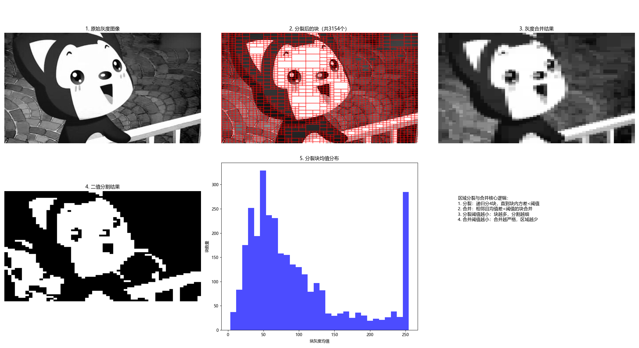
10.5 基于形态学分水岭的分割
10.5.1 背景知识
分水岭算法将图像视为地形地貌:
- 灰度值低的区域:山谷;
- 灰度值高的区域:山峰;
- 从山谷开始 "注水",不同山谷的水相遇时构建堤坝,最终堤坝即为分割边界。
10.5.2 堤坝构建
堤坝是分水岭分割的核心,本质是不同区域的边界,构建准则:
- 注水过程中,当两个不同区域的水即将汇合时,在汇合处构建堤坝;
- 堤坝的高度为当前注水高度,确保水不会混合。
10.5.3 分水岭分割算法
完整代码(含效果对比)
python
import cv2
import numpy as np
import matplotlib.pyplot as plt
import os

# ===================== 核心配置项 =====================
# 替换为你的图像路径(建议用coins.jpg或含多个独立目标的图像)
IMAGE_PATH = r"../picture/XueNai.png"
# 分水岭关键参数(可根据图像调整)
GAUSSIAN_KERNEL = (5, 5)  # 高斯模糊核大小
MORPH_KERNEL_SIZE = 3  # 形态学核大小
OPEN_ITERATIONS = 2  # 开运算迭代次数
DILATE_ITERATIONS = 3  # 膨胀迭代次数(确定背景)
DISTANCE_THRESH_RATIO = 0.7  # 距离变换阈值比例(确定前景)
# 显示窗口尺寸
FIG_SIZE = (22, 12)
# ======================================================

# 设置matplotlib支持中文显示
plt.rcParams['font.sans-serif'] = ['Microsoft YaHei', 'SimHei', 'DejaVu Sans']
plt.rcParams['axes.unicode_minus'] = False
plt.rcParams['font.family'] = 'sans-serif'


def watershed_segmentation(img_gray,
                           gaussian_kernel=(5, 5),
                           morph_kernel_size=3,
                           open_iter=2,
                           dilate_iter=3,
                           dist_thresh_ratio=0.7):
    """
    形态学分水岭分割(优化版)
    核心原理:
    1. 预处理:去噪+二值化,得到初始前景/背景
    2. 距离变换:精准定位前景核心区域
    3. 标记未知区域:背景-前景的过渡区
    4. 分水岭算法:基于标记的分割,避免过分割
    :param img_gray: 输入灰度图像
    :param gaussian_kernel: 高斯模糊核
    :param morph_kernel_size: 形态学操作核大小
    :param open_iter: 开运算迭代次数
    :param dilate_iter: 膨胀迭代次数
    :param dist_thresh_ratio: 距离变换阈值比例(0~1)
    :return:
        ws_color: 带分割边界的彩色图(红色为边界)
        markers: 标记矩阵
        process_steps: 预处理步骤结果(用于可视化)
    """
    # 1. 噪声去除(高斯模糊)
    blur = cv2.GaussianBlur(img_gray, gaussian_kernel, 0)

    # 2. 二值化(反相OTSU,使前景为白色,背景为黑色)
    _, thresh = cv2.threshold(blur, 0, 255, cv2.THRESH_BINARY_INV + cv2.THRESH_OTSU)

    # 3. 形态学开运算(先腐蚀后膨胀,去除小噪声点)
    kernel = np.ones((morph_kernel_size, morph_kernel_size), np.uint8)
    opening = cv2.morphologyEx(thresh, cv2.MORPH_OPEN, kernel, iterations=open_iter)

    # 4. 确定背景区域(膨胀操作,扩大背景范围)
    sure_bg = cv2.dilate(opening, kernel, iterations=dilate_iter)

    # 5. 确定前景区域(距离变换 + 阈值)
    # 距离变换:计算每个前景像素到最近背景的距离
    dist_transform = cv2.distanceTransform(opening, cv2.DIST_L2, 5)
    # 阈值筛选:保留距离变换值大的区域(前景核心)
    dist_thresh = dist_thresh_ratio * dist_transform.max()
    _, sure_fg = cv2.threshold(dist_transform, dist_thresh, 255, 0)
    sure_fg = np.uint8(sure_fg)

    # 6. 找到未知区域(背景 - 前景,即过渡区)
    unknown = cv2.subtract(sure_bg, sure_fg)

    # 7. 标记连通区域(为分水岭做准备)
    # 步骤7.1:连通组件分析(标记前景)
    num_labels, markers = cv2.connectedComponents(sure_fg)
    # 步骤7.2:调整标记(背景标记为1,前景从2开始,避免与0冲突)
    markers += 1
    # 步骤7.3:未知区域标记为0(分水岭算法会填充这些区域)
    markers[unknown == 255] = 0

    # 8. 分水岭分割(需要彩色图像输入)
    img_color = cv2.cvtColor(img_gray, cv2.COLOR_GRAY2BGR)
    markers = cv2.watershed(img_color, markers)

    # 9. 标记分割边界(标记为-1的区域是分割边界,标为红色)
    ws_color = img_color.copy()
    ws_color[markers == -1] = [0, 0, 255]  # BGR格式:红色

    # 存储预处理步骤(用于可视化)
    process_steps = {
        'blur': blur,
        'thresh': thresh,
        'opening': opening,
        'sure_bg': sure_bg,
        'dist_transform': dist_transform,
        'sure_fg': sure_fg,
        'unknown': unknown
    }

    return ws_color, markers, process_steps


def main():
    # 1. 加载灰度图像
    if not os.path.exists(IMAGE_PATH):
        print(f"警告:图像路径 {IMAGE_PATH} 不存在,使用内置coins测试图")
        img_gray = cv2.imread(cv2.samples.findFile('coins.jpg'), 0)
    else:
        img_gray = cv2.imread(IMAGE_PATH, 0)

    # 检查图像是否加载成功
    if img_gray is None:
        raise ValueError("无法加载图像,请检查路径或确保coins.jpg存在")

    # 2. 执行分水岭分割
    ws_color, markers, process_steps = watershed_segmentation(
        img_gray,
        gaussian_kernel=GAUSSIAN_KERNEL,
        morph_kernel_size=MORPH_KERNEL_SIZE,
        open_iter=OPEN_ITERATIONS,
        dilate_iter=DILATE_ITERATIONS,
        dist_thresh_ratio=DISTANCE_THRESH_RATIO
    )

    # 3. 可视化结果(分步展示,更易理解)
    plt.figure(figsize=FIG_SIZE)

    # 子图1:原始图像
    plt.subplot(3, 3, 1)
    plt.imshow(img_gray, cmap='gray')
    plt.title('1. 原始灰度图像', fontsize=10)
    plt.axis('off')

    # 子图2:高斯模糊去噪
    plt.subplot(3, 3, 2)
    plt.imshow(process_steps['blur'], cmap='gray')
    plt.title('2. 高斯模糊去噪', fontsize=10)
    plt.axis('off')

    # 子图3:OTSU二值化(反相)
    plt.subplot(3, 3, 3)
    plt.imshow(process_steps['thresh'], cmap='gray')
    plt.title('3. OTSU二值化(反相)', fontsize=10)
    plt.axis('off')

    # 子图4:形态学开运算
    plt.subplot(3, 3, 4)
    plt.imshow(process_steps['opening'], cmap='gray')
    plt.title('4. 开运算(去小噪声)', fontsize=10)
    plt.axis('off')

    # 子图5:确定背景(膨胀)
    plt.subplot(3, 3, 5)
    plt.imshow(process_steps['sure_bg'], cmap='gray')
    plt.title('5. 确定背景(膨胀)', fontsize=10)
    plt.axis('off')

    # 子图6:距离变换
    plt.subplot(3, 3, 6)
    plt.imshow(process_steps['dist_transform'], cmap='jet')
    plt.colorbar(shrink=0.6)
    plt.title('6. 距离变换', fontsize=10)
    plt.axis('off')

    # 子图7:确定前景(距离阈值)
    plt.subplot(3, 3, 7)
    plt.imshow(process_steps['sure_fg'], cmap='gray')
    plt.title('7. 确定前景(距离阈值)', fontsize=10)
    plt.axis('off')

    # 子图8:未知区域(背景-前景)
    plt.subplot(3, 3, 8)
    plt.imshow(process_steps['unknown'], cmap='gray')
    plt.title('8. 未知区域(过渡区)', fontsize=10)
    plt.axis('off')

    # 子图9:最终分割结果
    plt.subplot(3, 3, 9)
    plt.imshow(cv2.cvtColor(ws_color, cv2.COLOR_BGR2RGB))
    plt.title('9. 分水岭分割结果(红色=边界)', fontsize=10)
    plt.axis('off')

    plt.tight_layout()
    plt.show()

    # 打印关键信息
    num_objects = len(np.unique(markers)) - 2  # 减去背景(1)和边界(-1)
    print(f"分割出的目标数量:{num_objects}")
    print(
        f"距离变换阈值:{DISTANCE_THRESH_RATIO} × 最大值 = {DISTANCE_THRESH_RATIO * process_steps['dist_transform'].max():.2f}")


if __name__ == "__main__":
    main()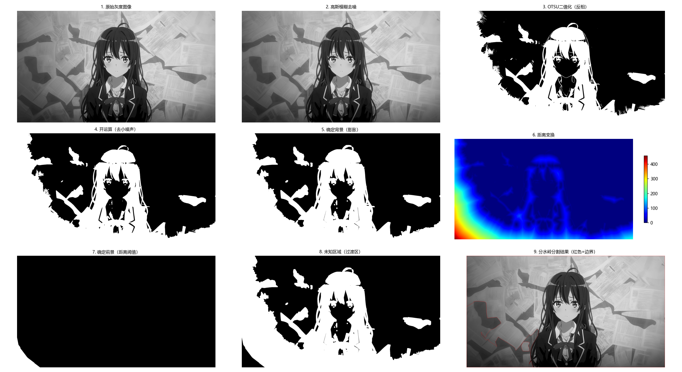
10.5.4 标记点的使用
标记点可避免分水岭算法的 "过分割" 问题,核心是手动 / 自动标记前景和背景种子点,引导分割方向。
完整代码(含效果对比)
python
import cv2
import numpy as np
import matplotlib.pyplot as plt
import os

# ===================== 核心配置项 =====================
# 替换为你的图像路径
IMAGE_PATH = r"../picture/KaTiXiYa.png"
# 交互选点开关(True=鼠标选点,False=使用预设标记点)
USE_MOUSE_MARKERS = True
# 预设标记点(仅当USE_MOUSE_MARKERS=False时生效)
PRESET_FG_MARKERS = [(50, 50), (100, 50), (150, 50), (50, 100), (100, 100)]
PRESET_BG_MARKERS = [(10, 10), (200, 200), (200, 10)]
# 预处理参数(提升分割效果)
GAUSSIAN_KERNEL = (3, 3)  # 高斯模糊核
MORPH_KERNEL = np.ones((3, 3), np.uint8)  # 形态学核
# 显示配置
FIG_SIZE = (20, 8)
# ======================================================

# 设置matplotlib中文显示
plt.rcParams['font.sans-serif'] = ['Microsoft YaHei', 'SimHei', 'DejaVu Sans']
plt.rcParams['axes.unicode_minus'] = False
plt.rcParams['font.family'] = 'sans-serif'

# 全局变量:存储鼠标选择的标记点
mouse_fg_markers = []
mouse_bg_markers = []
mouse_img = None


def mouse_callback(event, x, y, flags, param):
    """
    鼠标回调函数:
    - 左键点击:添加前景标记点(红色)
    - 右键点击:添加背景标记点(蓝色)
    - 滚轮点击/中键:清除所有标记点
    """
    global mouse_fg_markers, mouse_bg_markers, mouse_img
    if event == cv2.EVENT_LBUTTONDOWN:
        # 添加前景标记点
        mouse_fg_markers.append((x, y))
        cv2.circle(mouse_img, (x, y), 5, (0, 0, 255), -1)  # 红色实心圆
        cv2.putText(mouse_img, f'FG{len(mouse_fg_markers)}', (x + 8, y + 3),
                    cv2.FONT_HERSHEY_SIMPLEX, 0.4, (0, 0, 255), 1)
        print(f"添加前景标记点:({x}, {y})")
    elif event == cv2.EVENT_RBUTTONDOWN:
        # 添加背景标记点
        mouse_bg_markers.append((x, y))
        cv2.circle(mouse_img, (x, y), 5, (255, 0, 0), -1)  # 蓝色实心圆
        cv2.putText(mouse_img, f'BG{len(mouse_bg_markers)}', (x + 8, y + 3),
                    cv2.FONT_HERSHEY_SIMPLEX, 0.4, (255, 0, 0), 1)
        print(f"添加背景标记点:({x}, {y})")
    elif event == cv2.EVENT_MBUTTONDOWN:
        # 清除所有标记点
        mouse_fg_markers.clear()
        mouse_bg_markers.clear()
        mouse_img = param.copy()  # 重置图像
        print("已清除所有标记点")
    cv2.imshow("标记点选择(左键=前景,右键=背景,中键=清除,按ESC确认)", mouse_img)


def select_markers_interactively(img_gray):
    """
    交互式选择前景/背景标记点
    """
    global mouse_fg_markers, mouse_bg_markers, mouse_img
    # 重置标记点
    mouse_fg_markers = []
    mouse_bg_markers = []
    # 转为彩色图像用于标记
    mouse_img = cv2.cvtColor(img_gray, cv2.COLOR_GRAY2BGR)
    cv2.namedWindow("标记点选择(左键=前景,右键=背景,中键=清除,按ESC确认)", cv2.WINDOW_NORMAL)
    cv2.setMouseCallback("标记点选择(左键=前景,右键=背景,中键=清除,按ESC确认)",
                         mouse_callback, img_gray)

    print("===== 标记点选择指南 =====")
    print("1. 左键点击:添加前景标记点(目标区域,如硬币中心)")
    print("2. 右键点击:添加背景标记点(非目标区域,如空白背景)")
    print("3. 中键/滚轮点击:清除所有标记点")
    print("4. 按ESC键确认选择并退出")
    print("==========================")

    while True:
        cv2.imshow("标记点选择(左键=前景,右键=背景,中键=清除,按ESC确认)", mouse_img)
        key = cv2.waitKey(1) & 0xFF
        if key == 27:  # ESC键退出
            break
    cv2.destroyAllWindows()

    return mouse_fg_markers, mouse_bg_markers


def watershed_with_markers(img_gray, fg_markers, bg_markers, preprocess=True):
    """
    带标记点的分水岭分割(修复版)
    :param img_gray: 输入灰度图像
    :param fg_markers: 前景标记点列表 [(x1,y1), ...]
    :param bg_markers: 背景标记点列表 [(x1,y1), ...]
    :param preprocess: 是否进行预处理(去噪+形态学)
    :return:
        ws_color: 带分割边界的彩色图
        markers: 标记矩阵
        img_preprocessed: 预处理后的图像
    """
    # 步骤1:预处理(提升分割效果)
    if preprocess:
        # 高斯模糊去噪
        img_preprocessed = cv2.GaussianBlur(img_gray, GAUSSIAN_KERNEL, 0)
        # 形态学闭运算(填充小空洞)
        img_preprocessed = cv2.morphologyEx(img_preprocessed, cv2.MORPH_CLOSE, MORPH_KERNEL, iterations=1)
    else:
        img_preprocessed = img_gray.copy()

    # 步骤2:有效性检查
    if not fg_markers or not bg_markers:
        raise ValueError("前景和背景标记点都不能为空!")

    # 步骤3:初始化标记图(必须为int32类型,分水岭要求)
    markers = np.zeros_like(img_gray, dtype=np.int32)

    # 步骤4:标记前景(值=2)和背景(值=1)
    # 前景标记:扩展为小区域,避免单点标记不稳定
    for (x, y) in fg_markers:
        if 0 <= x < img_gray.shape[1] and 0 <= y < img_gray.shape[0]:
            cv2.circle(markers, (x, y), 3, 2, -1)  # 前景标记扩展为3px圆

    # 背景标记:扩展为小区域
    for (x, y) in bg_markers:
        if 0 <= x < img_gray.shape[1] and 0 <= y < img_gray.shape[0]:
            cv2.circle(markers, (x, y), 3, 1, -1)  # 背景标记扩展为3px圆

    # 步骤5:执行分水岭分割
    img_color = cv2.cvtColor(img_preprocessed, cv2.COLOR_GRAY2BGR)
    markers = cv2.watershed(img_color, markers)

    # 步骤6:标记分割边界和前景区域(修复核心:改用逐像素赋值,避免尺寸不匹配)
    ws_color = img_color.copy()
    # 1. 分割边界(标记值=-1)→ 红色
    ws_color[markers == -1] = [0, 0, 255]

    # 2. 前景区域(标记值>1)→ 绿色半透明(修复版)
    fg_mask = (markers > 1)
    # 创建绿色蒙版
    green_mask = np.zeros_like(ws_color)
    green_mask[fg_mask] = [0, 255, 0]  # 绿色
    # 混合原图和绿色蒙版(实现半透明效果)
    ws_color = cv2.addWeighted(ws_color, 0.7, green_mask, 0.3, 0)

    return ws_color, markers, img_preprocessed


def main():
    # 1. 加载灰度图像
    if not os.path.exists(IMAGE_PATH):
        print(f"警告:图像路径 {IMAGE_PATH} 不存在,使用内置coins测试图")
        img_gray = cv2.imread(cv2.samples.findFile('coins.jpg'), 0)
    else:
        img_gray = cv2.imread(IMAGE_PATH, 0)

    if img_gray is None:
        raise ValueError("无法加载图像,请检查路径是否正确!")

    # 2. 选择标记点(交互/预设)
    if USE_MOUSE_MARKERS:
        fg_markers, bg_markers = select_markers_interactively(img_gray)
        print(f"\n最终选择:前景标记点{len(fg_markers)}个,背景标记点{len(bg_markers)}个")
    else:
        fg_markers = PRESET_FG_MARKERS
        bg_markers = PRESET_BG_MARKERS
        print(f"使用预设标记点:前景{len(fg_markers)}个,背景{len(bg_markers)}个")

    # 3. 执行带标记的分水岭分割
    ws_color, markers, img_preprocessed = watershed_with_markers(
        img_gray, fg_markers, bg_markers, preprocess=True
    )

    # 4. 可视化结果
    plt.figure(figsize=FIG_SIZE)

    # 子图1:原始图像+标记点
    plt.subplot(1, 3, 1)
    plt.imshow(img_gray, cmap='gray')
    # 绘制前景标记点
    if fg_markers:
        plt.scatter([x for x, y in fg_markers], [y for x, y in fg_markers],
                    color='red', s=60, marker='o', label='前景标记')
    # 绘制背景标记点
    if bg_markers:
        plt.scatter([x for x, y in bg_markers], [y for x, y in bg_markers],
                    color='blue', s=60, marker='s', label='背景标记')
    plt.title('原始图像 + 标记点', fontsize=12)
    plt.legend(loc='best')
    plt.axis('off')

    # 子图2:预处理后的图像
    plt.subplot(1, 3, 2)
    plt.imshow(img_preprocessed, cmap='gray')
    plt.title('预处理后图像(去噪+闭运算)', fontsize=12)
    plt.axis('off')

    # 子图3:分水岭分割结果
    plt.subplot(1, 3, 3)
    plt.imshow(cv2.cvtColor(ws_color, cv2.COLOR_BGR2RGB))
    plt.title('带标记点的分水岭分割结果\n(红色=边界,绿色=前景)', fontsize=12)
    plt.axis('off')

    plt.tight_layout()
    plt.show()

    # 输出分割统计信息
    num_objects = len(np.unique(markers)) - 2  # 减去背景(1)和边界(-1)
    print(f"\n===== 分割结果统计 =====")
    print(f"检测到的目标数量:{num_objects}")
    print(f"标记点总数:前景{len(fg_markers)}个,背景{len(bg_markers)}个")
    print(f"标记矩阵取值范围:{np.min(markers)} ~ {np.max(markers)}")


if __name__ == "__main__":
    main()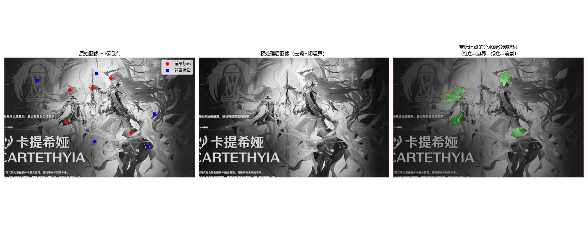
10.6 基于运动信息的分割
10.6.1 空间域方法
空间域运动分割主要基于帧间差分法:计算相邻两帧图像的灰度差,阈值化后得到运动区域。
完整代码(视频帧分割示例)
python
import cv2
import numpy as np
import os

# ===================== 核心配置项 =====================
# 视频路径(为空则使用摄像头)
VIDEO_PATH = r"C:\Users\王炳\Desktop\数字图像处理\课程设计\崩坏星穹铁道角色检测系统\StarRail_CNN_Detector\检测样本\视频\XiLian_PV.mp4"  # 替换为你的视频路径,或设为""使用摄像头
# 帧间差分参数
DIFF_THRESHOLD = 25  # 差分阈值(越小越灵敏,易检测小运动;越大越稳定,抗噪)
GAUSSIAN_KERNEL = (5, 5)  # 高斯模糊核(去噪)
MORPH_KERNEL_SIZE = 5  # 形态学核大小
MORPH_ITERATIONS = 1  # 形态学迭代次数
# 显示配置
WINDOW_SIZE = (800, 600)  # 显示窗口尺寸
FPS = 30  # 显示帧率(匹配视频/摄像头)


# ======================================================

def frame_diff_segmentation(video_path="",
                            diff_threshold=25,  # 修复:变量名改为diff_threshold,避免冲突
                            gaussian_kernel=(5, 5),
                            morph_kernel_size=5,
                            morph_iter=1,
                            show_fps=True):
    """
    帧间差分法(空间域运动分割)- 修复版
    核心原理:通过计算相邻帧的灰度差,检测像素级的运动变化,实现运动目标分割
    :param video_path: 视频路径(为空则使用摄像头)
    :param diff_threshold: 差分阈值(0-255)
    :param gaussian_kernel: 高斯模糊核
    :param morph_kernel_size: 形态学核大小
    :param morph_iter: 形态学迭代次数
    :param show_fps: 是否显示帧率
    :return: None(实时显示)
    """
    # ========== 1. 初始化视频/摄像头 ==========
    # 优先级:指定视频路径 > 摄像头
    if video_path and os.path.exists(video_path):
        cap = cv2.VideoCapture(video_path)
        print(f"正在加载视频:{video_path}")
    else:
        if video_path:
            print(f"视频路径不存在:{video_path},切换到摄像头")
        cap = cv2.VideoCapture(0)
        print("正在使用摄像头采集画面")

    # 检查视频/摄像头是否打开
    if not cap.isOpened():
        raise ValueError("无法打开视频文件或摄像头!")

    # 获取视频基本信息
    fps = cap.get(cv2.CAP_PROP_FPS) if cap.get(cv2.CAP_PROP_FPS) > 0 else FPS
    width = int(cap.get(cv2.CAP_PROP_FRAME_WIDTH))
    height = int(cap.get(cv2.CAP_PROP_FRAME_HEIGHT))
    print(f"视频/摄像头信息:分辨率 {width}×{height},帧率 {fps:.1f}")

    # ========== 2. 初始化第一帧 ==========
    # 循环读取,确保获取有效帧(避免第一帧为空)
    ret, prev_frame = cap.read()
    frame_count = 0
    start_time = cv2.getTickCount()

    while not ret and cap.isOpened():
        ret, prev_frame = cap.read()
        frame_count += 1
        if frame_count > 10:  # 最多尝试10次
            raise ValueError("无法读取视频/摄像头的有效帧!")

    # 预处理第一帧:灰度化 + 高斯模糊(去噪)
    prev_gray = cv2.cvtColor(prev_frame, cv2.COLOR_BGR2GRAY)
    prev_gray = cv2.GaussianBlur(prev_gray, gaussian_kernel, 0)

    # 创建形态学核
    morph_kernel = np.ones((morph_kernel_size, morph_kernel_size), np.uint8)

    # ========== 3. 帧间差分主循环 ==========
    while cap.isOpened():
        ret, curr_frame = cap.read()
        if not ret:
            print("视频播放完毕/摄像头采集结束")
            break

        # 调整显示窗口尺寸
        curr_frame_resized = cv2.resize(curr_frame, WINDOW_SIZE)
        prev_frame_resized = cv2.resize(prev_frame, WINDOW_SIZE)

        # ========== 4. 预处理当前帧 ==========
        curr_gray = cv2.cvtColor(curr_frame, cv2.COLOR_BGR2GRAY)
        curr_gray = cv2.GaussianBlur(curr_gray, gaussian_kernel, 0)

        # ========== 5. 核心:帧间差分 ==========
        # 计算相邻帧的绝对差值
        diff = cv2.absdiff(prev_gray, curr_gray)
        # 阈值化:提取运动区域(二值化)
        # 修复:变量名改为diff_binary,避免和阈值参数冲突
        _, diff_binary = cv2.threshold(diff, diff_threshold, 255, cv2.THRESH_BINARY)
        # 形态学闭运算:先膨胀后腐蚀,填充小空洞、连接断裂区域
        diff_binary = cv2.morphologyEx(diff_binary, cv2.MORPH_CLOSE, morph_kernel, iterations=morph_iter)
        # 可选:开运算去除小噪声点
        diff_binary = cv2.morphologyEx(diff_binary, cv2.MORPH_OPEN, morph_kernel, iterations=morph_iter)

        # ========== 6. 结果增强 ==========
        # 1. 标记运动区域(红色)
        curr_frame_marked = curr_frame_resized.copy()
        diff_binary_resized = cv2.resize(diff_binary, WINDOW_SIZE)
        curr_frame_marked[diff_binary_resized == 255] = [0, 0, 255]  # BGR:红色

        # 2. 计算运动区域占比
        motion_pixels = np.sum(diff_binary > 0)
        total_pixels = diff_binary.shape[0] * diff_binary.shape[1]
        motion_ratio = (motion_pixels / total_pixels) * 100

        # 3. 显示帧率(可选)
        if show_fps:
            frame_count += 1
            elapsed_time = (cv2.getTickCount() - start_time) / cv2.getTickFrequency()
            current_fps = frame_count / elapsed_time if elapsed_time > 0 else 0
            cv2.putText(curr_frame_marked, f"FPS: {current_fps:.1f}", (10, 30),
                        cv2.FONT_HERSHEY_SIMPLEX, 1, (0, 255, 0), 2)

        # 4. 显示运动区域占比
        cv2.putText(curr_frame_marked, f"Motion: {motion_ratio:.1f}%", (10, 70),
                    cv2.FONT_HERSHEY_SIMPLEX, 1, (255, 255, 0), 2)

        # ========== 7. 显示结果 ==========
        # 组合显示窗口:原始帧 + 差分图 + 标记帧
        diff_binary_color = cv2.cvtColor(diff_binary_resized, cv2.COLOR_GRAY2BGR)
        combined_frame = np.hstack((prev_frame_resized, diff_binary_color, curr_frame_marked))

        # 调整组合窗口尺寸(避免过大)
        combined_height = WINDOW_SIZE[1]
        combined_width = WINDOW_SIZE[0] * 3
        if combined_width > 1920:  # 限制最大宽度
            scale = 1920 / combined_width
            combined_frame = cv2.resize(combined_frame, (int(combined_width * scale), int(combined_height * scale)))

        cv2.imshow('Frame Difference Segmentation (Prev | Diff | Marked)', combined_frame)

        # ========== 8. 更新状态 ==========
        prev_gray = curr_gray
        prev_frame = curr_frame

        # 按q/ESC退出,按空格暂停
        key = cv2.waitKey(int(1000 / fps)) & 0xFF
        if key == ord('q') or key == 27:  # q/ESC
            print("用户手动退出")
            break
        elif key == ord(' '):  # 空格暂停
            cv2.waitKey(0)  # 按任意键继续

    # ========== 9. 资源释放 ==========
    cap.release()
    cv2.destroyAllWindows()
    print("资源已释放,程序结束")


# ========== 主函数:运行帧间差分分割 ==========
if __name__ == "__main__":
    try:
        frame_diff_segmentation(
            video_path=VIDEO_PATH,
            diff_threshold=DIFF_THRESHOLD,  # 同步修改参数名
            gaussian_kernel=GAUSSIAN_KERNEL,
            morph_kernel_size=MORPH_KERNEL_SIZE,
            morph_iter=MORPH_ITERATIONS,
            show_fps=True
        )
    except Exception as e:
        print(f"程序运行出错:{e}")
        cv2.destroyAllWindows()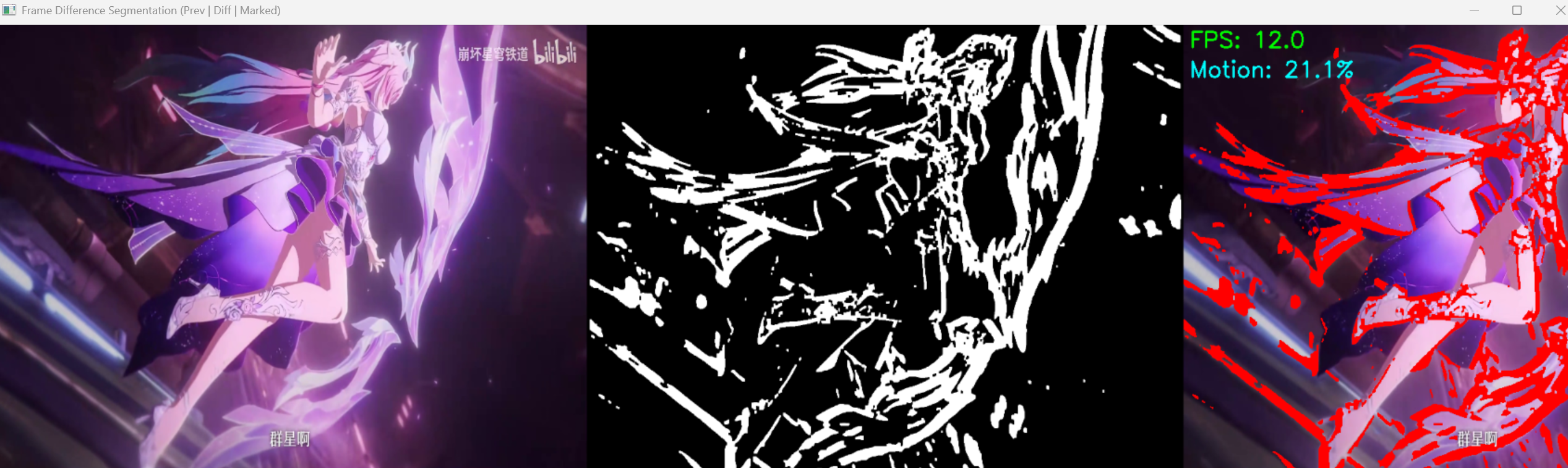
10.6.2 频域方法
频域运动分割基于傅里叶变换:将视频帧转换到频域,分析频率分量的变化,提取运动信息(简化版示例)。
完整代码
python
import cv2
import numpy as np
import matplotlib.pyplot as plt
import os

plt.rcParams['font.sans-serif'] = ['SimHei']
plt.rcParams['axes.unicode_minus'] = False
# ===================== 核心配置项 =====================
# 图像路径(为空则使用Lena模拟帧)
FRAME1_PATH = r"../picture/KaTiXiYa.png"
FRAME2_PATH = r"../picture/JinXi.png"
# 频域分割参数
FREQ_THRESHOLD = 10  # 幅度谱差阈值(0-255)
GAUSSIAN_KERNEL = (3, 3)  # 高斯模糊核(去噪)
MORPH_KERNEL_SIZE = 5  # 形态学核大小
# 显示配置
FIG_SIZE = (18, 8)


# ======================================================

def frequency_domain_segmentation(frame1, frame2,
                                  freq_thresh=10,
                                  gaussian_kernel=(3, 3),
                                  morph_kernel_size=5,
                                  use_phase=False):
    """
    频域运动分割(优化版)
    核心原理:
    1. 傅里叶变换将图像从空间域转为频域,运动体现为频域幅度/相位的变化
    2. 计算两帧频域幅度谱(或相位谱)的差异,阈值化提取运动区域
    :param frame1: 帧1(灰度图)
    :param frame2: 帧2(灰度图)
    :param freq_thresh: 频域差值阈值
    :param gaussian_kernel: 高斯模糊核(预处理去噪)
    :param morph_kernel_size: 形态学核大小(后处理优化)
    :param use_phase: 是否使用相位谱(默认用幅度谱,相位谱对运动更敏感)
    :return:
        motion_seg: 二值化运动区域
        mag1: 帧1幅度谱(可视化用)
        mag2: 帧2幅度谱(可视化用)
        mag_diff: 幅度谱差值(可视化用)
    """
    # ========== 1. 预处理:去噪 + 统一尺寸 ==========
    # 确保两帧尺寸一致
    if frame1.shape != frame2.shape:
        frame2 = cv2.resize(frame2, (frame1.shape[1], frame1.shape[0]))

    # 高斯模糊去噪(减少频域噪声)
    frame1_blur = cv2.GaussianBlur(frame1, gaussian_kernel, 0)
    frame2_blur = cv2.GaussianBlur(frame2, gaussian_kernel, 0)

    # ========== 2. 傅里叶变换 ==========
    # 快速傅里叶变换(FFT)
    f1 = np.fft.fft2(frame1_blur)
    f2 = np.fft.fft2(frame2_blur)

    # 移频:将低频分量移到中心(便于分析)
    f1_shift = np.fft.fftshift(f1)
    f2_shift = np.fft.fftshift(f2)

    # ========== 3. 计算频域特征 ==========
    # 幅度谱(反映亮度/能量分布)
    mag1 = np.abs(f1_shift)
    mag2 = np.abs(f2_shift)
    # 幅度谱对数缩放(便于可视化)
    mag1_log = 20 * np.log(mag1 + 1e-8)  # +1e-8避免log(0)
    mag2_log = 20 * np.log(mag2 + 1e-8)

    # 相位谱(反映位置/运动信息)
    phase1 = np.angle(f1_shift)
    phase2 = np.angle(f2_shift)

    # ========== 4. 计算频域差值 ==========
    if use_phase:
        # 相位谱差值(对运动更敏感)
        freq_diff = cv2.absdiff(phase1, phase2)
        # 归一化到0-255
        freq_diff = cv2.normalize(freq_diff, None, 0, 255, cv2.NORM_MINMAX)
    else:
        # 幅度谱差值(更稳定,抗光照变化)
        freq_diff = cv2.absdiff(mag1_log, mag2_log)

    # ========== 5. 后处理:阈值化 + 形态学操作 ==========
    # 转换为8位无符号整数(OpenCV要求)
    freq_diff_uint8 = np.uint8(freq_diff)
    # 阈值化提取运动区域
    _, motion_seg = cv2.threshold(freq_diff_uint8, freq_thresh, 255, cv2.THRESH_BINARY)

    # 形态学操作优化(闭运算填充空洞,开运算去噪)
    morph_kernel = np.ones((morph_kernel_size, morph_kernel_size), np.uint8)
    motion_seg = cv2.morphologyEx(motion_seg, cv2.MORPH_CLOSE, morph_kernel)
    motion_seg = cv2.morphologyEx(motion_seg, cv2.MORPH_OPEN, morph_kernel)

    return motion_seg, mag1_log, mag2_log, freq_diff


def load_frames(frame1_path, frame2_path):
    """
    加载两帧图像,加载失败则生成模拟帧(Lena平移)
    """
    # 尝试加载指定图像
    frame1 = cv2.imread(frame1_path, 0) if frame1_path else None
    frame2 = cv2.imread(frame2_path, 0) if frame2_path else None

    # 加载失败则生成模拟帧
    if frame1 is None or frame2 is None:
        print(f"指定图像加载失败,使用Lena模拟运动帧")
        # 加载Lena测试图
        frame1 = cv2.imread(cv2.samples.findFile('lena.jpg'), 0)
        # 帧2:平移5像素 + 轻微亮度变化(模拟真实场景)
        frame2 = np.roll(frame1, 5, axis=1)  # 水平平移5像素
        frame2 = frame2.astype(np.float32) + 5  # 亮度+5
        frame2 = np.clip(frame2, 0, 255).astype(np.uint8)  # 限制范围

    return frame1, frame2


def visualize_results(frame1, frame2, motion_seg, mag1_log, mag2_log, freq_diff):
    """
    可视化频域分割结果
    """
    plt.figure(figsize=FIG_SIZE)

    # 子图1:原始帧1
    plt.subplot(2, 3, 1)
    plt.imshow(frame1, cmap='gray')
    plt.title('原始帧1', fontsize=12)
    plt.axis('off')

    # 子图2:原始帧2
    plt.subplot(2, 3, 2)
    plt.imshow(frame2, cmap='gray')
    plt.title('原始帧2(平移5像素)', fontsize=12)
    plt.axis('off')

    # 子图3:运动区域分割结果
    plt.subplot(2, 3, 3)
    plt.imshow(motion_seg, cmap='gray')
    plt.title('频域运动分割结果', fontsize=12)
    plt.axis('off')

    # 子图4:帧1幅度谱
    plt.subplot(2, 3, 4)
    plt.imshow(mag1_log, cmap='gray')
    plt.title('帧1频域幅度谱', fontsize=12)
    plt.axis('off')

    # 子图5:帧2幅度谱
    plt.subplot(2, 3, 5)
    plt.imshow(mag2_log, cmap='gray')
    plt.title('帧2频域幅度谱', fontsize=12)
    plt.axis('off')

    # 子图6:幅度谱差值
    plt.subplot(2, 3, 6)
    plt.imshow(freq_diff, cmap='jet')
    plt.title('频域差值(运动区域)', fontsize=12)
    plt.colorbar(shrink=0.8)
    plt.axis('off')

    plt.tight_layout()
    plt.show()


# ========== 主函数:运行频域运动分割 ==========
if __name__ == "__main__":
    try:
        # 1. 加载帧
        frame1, frame2 = load_frames(FRAME1_PATH, FRAME2_PATH)

        # 2. 频域运动分割
        motion_seg, mag1_log, mag2_log, freq_diff = frequency_domain_segmentation(
            frame1, frame2,
            freq_thresh=FREQ_THRESHOLD,
            gaussian_kernel=GAUSSIAN_KERNEL,
            morph_kernel_size=MORPH_KERNEL_SIZE,
            use_phase=False  # 设为True可使用相位谱(对运动更敏感)
        )

        # 3. 可视化结果
        visualize_results(frame1, frame2, motion_seg, mag1_log, mag2_log, freq_diff)

        # 4. 输出统计信息
        motion_pixels = np.sum(motion_seg > 0)
        total_pixels = motion_seg.shape[0] * motion_seg.shape[1]
        motion_ratio = (motion_pixels / total_pixels) * 100
        print(f"运动区域占比:{motion_ratio:.2f}%")
        print(f"频域差值范围:{np.min(freq_diff):.2f} ~ {np.max(freq_diff):.2f}")

    except Exception as e:
        print(f"程序运行出错:{e}")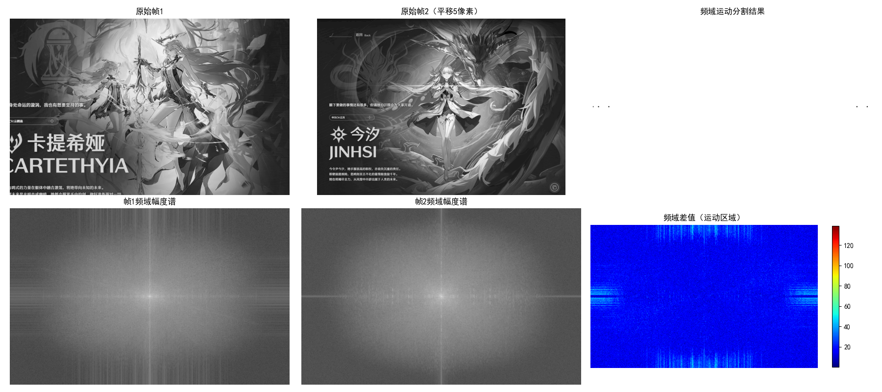
小结
图像分割是数字图像处理的核心技术,本文从基础到进阶,结合完整 Python 代码和效果对比图,讲解了图像分割的主要方法:
- 点线边缘检测:从孤立点、线到边缘,是分割的基础,Canny 算子是工业级标准;
- 阈值分割:最简单高效的分割方法,大津法可自动计算最优全局阈值,自适应阈值适用于光照不均匀场景;
- 区域分割:区域生长从种子点扩展,区域分裂与合并适合复杂纹理图像;
- 分水岭分割:基于形态学,标记点可解决过分割问题;
- 运动分割:帧间差分(空间域)和傅里叶变换(频域)是常用方法。
实际应用中,需根据图像特点选择合适的分割方法,或结合多种方法(如边缘检测 + 阈值分割)提升效果。
总结
- 核心方法分类:图像分割可分为基于灰度特征(点线边缘、阈值)、基于区域、基于形态学、基于运动信息四大类,不同方法适用于不同场景;
- 关键技巧:噪声去除(高斯平滑)可显著提升分割效果,标记点 / 种子点是解决过分割、引导分割方向的有效手段;
- 代码实战要点:所有代码均包含完整注释和效果对比,运行前需确保安装依赖库,替换测试图像 / 视频路径即可直接运行。