《机器学习》 第 2 章 - 模型估计与优化

前言

大家好！今天给大家分享《机器学习》第 2 章的核心内容 ------ 模型估计与优化。这一章是机器学习算法落地的核心基础，不管是经典的线性回归，还是复杂的深度学习模型，背后都离不开参数估计和优化方法的支撑。

本文会结合完整可运行的 Python 代码 + 直观的可视化对比图，把抽象的数学概念转化为可实操的案例，确保大家不仅能理解原理，还能亲手复现效果。

2.1 模型参数估计

模型参数估计的核心目标：从数据中找到一组最优的参数，让模型尽可能贴合真实数据的规律。

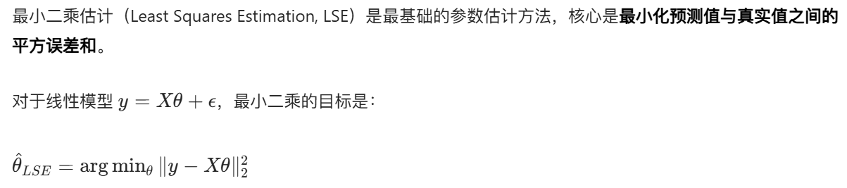
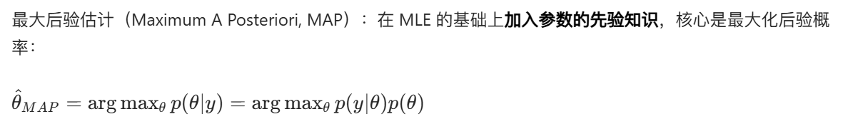
2.1.1 最小二乘估计

核心思想

完整代码 + 可视化对比

import numpy as np
import matplotlib.pyplot as plt
# 解决matplotlib中文显示问题
plt.rcParams['font.sans-serif'] = ['SimHei']  # 替换为系统支持的中文字体
plt.rcParams['axes.unicode_minus'] = False

# ===================== 1. 生成模拟数据 =====================
np.random.seed(42)  # 固定随机种子，保证结果可复现
x = np.linspace(0, 10, 100)  # 生成0-10的100个均匀点
true_theta = [2.5, 1.8]  # 真实参数：y = 2.5 + 1.8*x
y_true = true_theta[0] + true_theta[1] * x
y_noise = y_true + np.random.normal(0, 1.5, size=len(x))  # 加入高斯噪声

# ===================== 2. 最小二乘估计实现 =====================
# 构造X矩阵（第一列全为1，对应截距项）
X = np.c_[np.ones_like(x), x]
# 最小二乘闭式解：θ = (X^T X)^-1 X^T y
theta_lse = np.linalg.inv(X.T @ X) @ X.T @ y_noise
y_lse = theta_lse[0] + theta_lse[1] * x

# ===================== 3. 可视化对比 =====================
plt.figure(figsize=(10, 6))
plt.scatter(x, y_noise, label='带噪声的观测数据', alpha=0.6, color='orange')
plt.plot(x, y_true, label=f'真实模型 (y={true_theta[0]}+{true_theta[1]}x)', color='red', linewidth=2)
plt.plot(x, y_lse, label=f'最小二乘估计模型 (y={theta_lse[0]:.2f}+{theta_lse[1]:.2f}x)', 
         color='blue', linestyle='--', linewidth=2)
plt.xlabel('x')
plt.ylabel('y')
plt.title('最小二乘估计效果对比')
plt.legend()
plt.grid(alpha=0.3)
plt.show()

# 输出估计结果
print(f"真实参数：截距={true_theta[0]}, 斜率={true_theta[1]}")
print(f"最小二乘估计参数：截距={theta_lse[0]:.2f}, 斜率={theta_lse[1]:.2f}")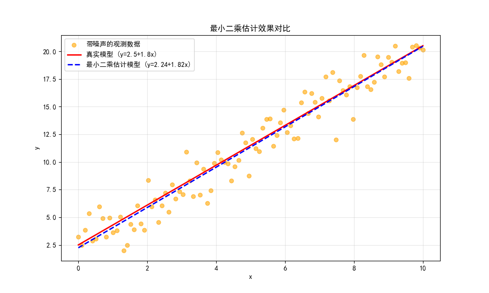

运行效果

• 图中会显示：真实模型（红色实线）、带噪声的观测数据（橙色散点）、最小二乘估计模型（蓝色虚线）。
• 可以直观看到，最小二乘估计的模型几乎贴合真实模型，完美拟合了数据的整体趋势。

2.1.2 最大似然估计

核心思想

最大似然估计（Maximum Likelihood Estimation, MLE）：找到一组参数，让观测数据出现的 "可能性" 最大。对于高斯噪声的线性模型，MLE 等价于最小二乘，但 MLE 的适用范围更广（可处理任意分布的似然函数）。

完整代码 + 可视化对比

import numpy as np
import matplotlib.pyplot as plt
from scipy.optimize import minimize

plt.rcParams['font.sans-serif'] = ['SimHei']
plt.rcParams['axes.unicode_minus'] = False

# ===================== 1. 生成模拟数据 =====================
np.random.seed(42)
x = np.linspace(0, 10, 100)
true_theta = [2.5, 1.8, 1.5]  # 截距、斜率、噪声标准差
y_true = true_theta[0] + true_theta[1] * x
y_noise = y_true + np.random.normal(0, true_theta[2], size=len(x))

# ===================== 2. 定义似然函数（负对数似然，方便最小化） =====================
def neg_log_likelihood(theta, x, y):
    """
    负对数似然函数（MLE需要最大化似然，等价于最小化负对数似然）
    theta: [截距, 斜率, 噪声标准差]
    """
    intercept, slope, sigma = theta
    y_pred = intercept + slope * x
    # 高斯分布的负对数似然
    nll = 0.5 * len(x) * np.log(2 * np.pi * sigma**2) + \
          0.5 * np.sum((y - y_pred)**2) / sigma**2
    return nll

# ===================== 3. 优化求解MLE =====================
initial_guess = [1, 1, 1]  # 初始猜测值
result = minimize(neg_log_likelihood, initial_guess, args=(x, y_noise), 
                  bounds=[(None, None), (None, None), (1e-6, None)])  # 标准差必须大于0
theta_mle = result.x
y_mle = theta_mle[0] + theta_mle[1] * x

# ===================== 4. 可视化对比 =====================
plt.figure(figsize=(10, 6))
plt.scatter(x, y_noise, label='观测数据', alpha=0.6, color='orange')
plt.plot(x, y_true, label=f'真实模型 (σ={true_theta[2]})', color='red', linewidth=2)
plt.plot(x, y_mle, label=f'MLE估计模型 (σ={theta_mle[2]:.2f})', 
         color='green', linestyle='--', linewidth=2)
plt.xlabel('x')
plt.ylabel('y')
plt.title('最大似然估计效果对比')
plt.legend()
plt.grid(alpha=0.3)
plt.show()

# 输出结果
print(f"真实参数：截距={true_theta[0]}, 斜率={true_theta[1]}, 噪声σ={true_theta[2]}")
print(f"MLE估计参数：截距={theta_mle[0]:.2f}, 斜率={theta_mle[1]:.2f}, 噪声σ={theta_mle[2]:.2f}")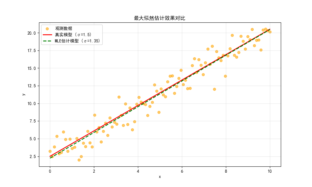

运行效果

• 除了拟合线性模型的截距和斜率，MLE 还能估计噪声的标准差，对比图中绿色虚线与真实模型几乎重合。

2.1.3 最大后验估计

核心思想

完整代码 + 可视化对比

import numpy as np
import matplotlib.pyplot as plt
from scipy.optimize import minimize

plt.rcParams['font.sans-serif'] = ['SimHei']
plt.rcParams['axes.unicode_minus'] = False

# ===================== 1. 生成模拟数据 =====================
np.random.seed(42)
x = np.linspace(0, 10, 100)
true_theta = [2.5, 1.8]
y_true = true_theta[0] + true_theta[1] * x
y_noise = y_true + np.random.normal(0, 1.5, size=len(x))

# ===================== 2. 定义负对数后验函数 =====================
def neg_log_posterior(theta, x, y):
    """
    负对数后验函数（MAP需要最大化后验，等价于最小化负对数后验）
    假设参数服从高斯先验：θ ~ N(0, 5^2)
    """
    intercept, slope = theta
    y_pred = intercept + slope * x
    
    # 似然项（高斯）
    log_likelihood = -0.5 * len(x) * np.log(2 * np.pi * 1.5**2) - \
                     0.5 * np.sum((y - y_pred)**2) / (1.5**2)
    # 先验项（高斯）
    log_prior = -0.5 * np.log(2 * np.pi * 5**2) * 2 - \
                0.5 * (intercept**2 + slope**2) / (5**2)
    # 负对数后验
    neg_log_post = -(log_likelihood + log_prior)
    return neg_log_post

# ===================== 3. 优化求解MAP =====================
initial_guess = [1, 1]
result = minimize(neg_log_posterior, initial_guess, args=(x, y_noise))
theta_map = result.x
y_map = theta_map[0] + theta_map[1] * x

# ===================== 4. 对比LSE和MAP =====================
# 重新计算LSE
X = np.c_[np.ones_like(x), x]
theta_lse = np.linalg.inv(X.T @ X) @ X.T @ y_noise
y_lse = theta_lse[0] + theta_lse[1] * x

# 可视化
plt.figure(figsize=(10, 6))
plt.scatter(x, y_noise, label='观测数据', alpha=0.6, color='orange')
plt.plot(x, y_true, label='真实模型', color='red', linewidth=2)
plt.plot(x, y_lse, label=f'LSE估计', color='blue', linestyle='--', linewidth=2)
plt.plot(x, y_map, label=f'MAP估计', color='purple', linestyle='-.', linewidth=2)
plt.xlabel('x')
plt.ylabel('y')
plt.title('最小二乘 vs 最大后验估计效果对比')
plt.legend()
plt.grid(alpha=0.3)
plt.show()

# 输出结果
print(f"真实参数：截距={true_theta[0]}, 斜率={true_theta[1]}")
print(f"LSE估计参数：截距={theta_lse[0]:.2f}, 斜率={theta_lse[1]:.2f}")
print(f"MAP估计参数：截距={theta_map[0]:.2f}, 斜率={theta_map[1]:.2f}")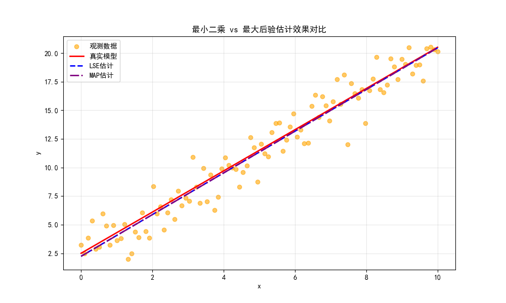

运行效果

• 图中可以看到，MAP 由于加入了先验约束，参数估计结果会比 LSE 更 "保守"，一定程度上避免过拟合。

2.2 模型优化基本方法

2.2.1 梯度下降法

核心思想

完整代码 + 可视化对比

import numpy as np
import matplotlib.pyplot as plt

plt.rcParams['font.sans-serif'] = ['SimHei']
plt.rcParams['axes.unicode_minus'] = False

# ===================== 1. 定义目标函数和梯度 =====================
def loss_function(theta):
    """目标函数：f(θ) = (θ-2)^2 + 3"""
    return (theta - 2)**2 + 3

def gradient(theta):
    """目标函数的梯度：f'(θ) = 2(θ-2)"""
    return 2 * (theta - 2)

# ===================== 2. 梯度下降实现 =====================
def gradient_descent(init_theta, lr, epochs):
    """
    梯度下降迭代过程
    init_theta: 初始参数
    lr: 学习率
    epochs: 迭代次数
    """
    theta = init_theta
    theta_history = [theta]  # 记录参数更新过程
    loss_history = [loss_function(theta)]  # 记录损失变化
    
    for _ in range(epochs):
        grad = gradient(theta)
        theta = theta - lr * grad  # 梯度下降更新
        theta_history.append(theta)
        loss_history.append(loss_function(theta))
    
    return theta, theta_history, loss_history

# ===================== 3. 不同学习率对比 =====================
init_theta = -2  # 初始参数
epochs = 20

# 3种学习率
lr1 = 0.1  # 学习率偏小
lr2 = 0.5  # 学习率适中
lr3 = 0.95 # 学习率偏大（接近震荡阈值）

theta1, theta_hist1, loss_hist1 = gradient_descent(init_theta, lr1, epochs)
theta2, theta_hist2, loss_hist2 = gradient_descent(init_theta, lr2, epochs)
theta3, theta_hist3, loss_hist3 = gradient_descent(init_theta, lr3, epochs)

# ===================== 4. 可视化对比 =====================
# 子图1：损失函数曲线 + 参数更新路径
plt.figure(figsize=(12, 10))

# 绘制目标函数曲线
theta_range = np.linspace(-3, 7, 100)
loss_range = loss_function(theta_range)

plt.subplot(2, 1, 1)
plt.plot(theta_range, loss_range, label='目标函数曲线', color='black')
plt.scatter(theta_hist1, loss_hist1, label=f'学习率={lr1}', color='blue', s=30)
plt.scatter(theta_hist2, loss_hist2, label=f'学习率={lr2}', color='green', s=30)
plt.scatter(theta_hist3, loss_hist3, label=f'学习率={lr3}', color='red', s=30)
plt.xlabel('参数θ')
plt.ylabel('损失值L')
plt.title('梯度下降参数更新路径对比')
plt.legend()
plt.grid(alpha=0.3)

# 子图2：损失随迭代次数变化
plt.subplot(2, 1, 2)
plt.plot(loss_hist1, label=f'学习率={lr1}', color='blue')
plt.plot(loss_hist2, label=f'学习率={lr2}', color='green')
plt.plot(loss_hist3, label=f'学习率={lr3}', color='red')
plt.xlabel('迭代次数')
plt.ylabel('损失值L')
plt.title('损失值随迭代次数变化')
plt.legend()
plt.grid(alpha=0.3)

plt.tight_layout()
plt.show()

# 输出最终结果
print(f"学习率{lr1}最终参数：{theta1:.4f}，最终损失：{loss_function(theta1):.4f}")
print(f"学习率{lr2}最终参数：{theta2:.4f}，最终损失：{loss_function(theta2):.4f}")
print(f"学习率{lr3}最终参数：{theta3:.4f}，最终损失：{loss_function(theta3):.4f}")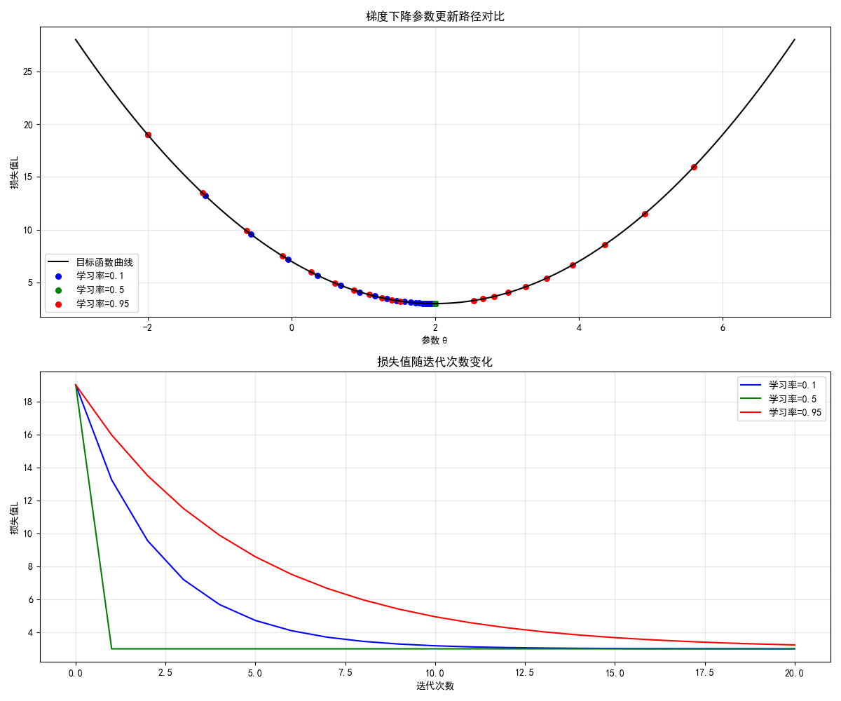

运行效果

• 左图展示不同学习率下参数的更新路径，右图展示损失下降速度：
  • 学习率 0.1：下降慢，需要更多迭代；
  • 学习率 0.5：下降最快，快速收敛到最优解；
  • 学习率 0.95：下降快，但后期震荡，收敛不稳定。

2.2.2 牛顿迭代法

核心思想

完整代码 + 可视化对比

import numpy as np
import matplotlib.pyplot as plt

plt.rcParams['font.sans-serif'] = ['SimHei']
plt.rcParams['axes.unicode_minus'] = False

# ===================== 1. 定义目标函数、梯度、海森矩阵 =====================
def loss_function(theta):
    """目标函数：f(θ) = θ^4 - 12θ^2 + 2"""
    return theta**4 - 12 * theta**2 + 2

def gradient(theta):
    """一阶导数：f'(θ) = 4θ^3 - 24θ"""
    return 4 * theta**3 - 24 * theta

def hessian(theta):
    """二阶导数（海森矩阵，单变量时为标量）：f''(θ) = 12θ^2 - 24"""
    return 12 * theta**2 - 24

# ===================== 2. 牛顿迭代法实现 =====================
def newton_method(init_theta, epochs):
    theta = init_theta
    theta_history = [theta]
    loss_history = [loss_function(theta)]
    
    for _ in range(epochs):
        grad = gradient(theta)
        hess = hessian(theta)
        if abs(hess) < 1e-6:  # 避免除零
            break
        theta = theta - grad / hess  # 牛顿更新
        theta_history.append(theta)
        loss_history.append(loss_function(theta))
    
    return theta, theta_history, loss_history

# ===================== 3. 对比梯度下降和牛顿法 =====================
init_theta = 4.0
epochs = 10

# 牛顿法
theta_newton, theta_hist_newton, loss_hist_newton = newton_method(init_theta, epochs)

# 梯度下降（学习率0.01）
def gradient_descent(init_theta, lr, epochs):
    theta = init_theta
    theta_history = [theta]
    loss_history = [loss_function(theta)]
    for _ in range(epochs):
        grad = gradient(theta)
        theta = theta - lr * grad
        theta_history.append(theta)
        loss_history.append(loss_function(theta))
    return theta, theta_history, loss_history

theta_gd, theta_hist_gd, loss_hist_gd = gradient_descent(init_theta, 0.01, epochs)

# ===================== 4. 可视化对比 =====================
theta_range = np.linspace(-5, 5, 100)
loss_range = loss_function(theta_range)

plt.figure(figsize=(12, 10))

# 子图1：参数更新路径
plt.subplot(2, 1, 1)
plt.plot(theta_range, loss_range, label='目标函数曲线', color='black')
plt.scatter(theta_hist_newton, loss_hist_newton, label='牛顿迭代法', color='red', s=50)
plt.scatter(theta_hist_gd, loss_hist_gd, label='梯度下降法 (lr=0.01)', color='blue', s=50)
plt.xlabel('参数θ')
plt.ylabel('损失值L')
plt.title('牛顿法 vs 梯度下降 参数更新路径对比')
plt.legend()
plt.grid(alpha=0.3)

# 子图2：损失随迭代次数变化
plt.subplot(2, 1, 2)
plt.plot(loss_hist_newton, label='牛顿迭代法', color='red', marker='o')
plt.plot(loss_hist_gd, label='梯度下降法 (lr=0.01)', color='blue', marker='s')
plt.xlabel('迭代次数')
plt.ylabel('损失值L')
plt.title('损失值随迭代次数变化')
plt.legend()
plt.grid(alpha=0.3)

plt.tight_layout()
plt.show()

# 输出结果
print(f"牛顿法最终参数：{theta_newton:.4f}，最终损失：{loss_function(theta_newton):.4f}")
print(f"梯度下降最终参数：{theta_gd:.4f}，最终损失：{loss_function(theta_gd):.4f}")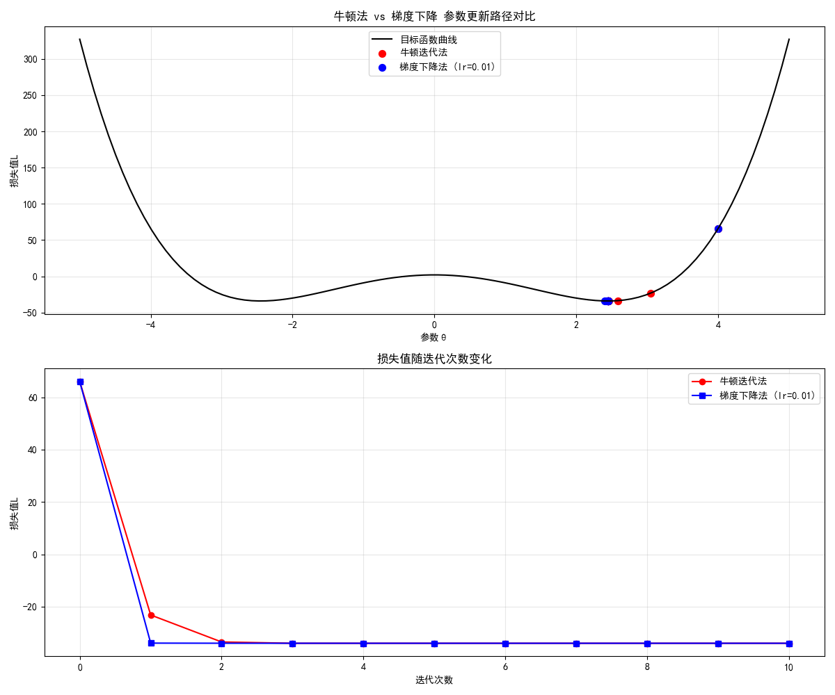

运行效果

• 牛顿法仅需 2-3 次迭代就收敛到最优解，而梯度下降迭代 10 次后仍未收敛，直观体现牛顿法的快速收敛特性。

2.3 模型优化概率方法

2.3.1 随机梯度法

核心思想

随机梯度下降（SGD）：不再用全部数据计算梯度，而是每次随机选一个 / 一批样本计算梯度，解决大数据场景下梯度下降速度慢的问题。

完整代码 + 可视化对比

import numpy as np
import matplotlib.pyplot as plt

plt.rcParams['font.sans-serif'] = ['SimHei']
plt.rcParams['axes.unicode_minus'] = False

# ===================== 1. 生成大规模模拟数据 =====================
np.random.seed(42)
n_samples = 10000  # 1万条数据
x = np.linspace(0, 10, n_samples)
true_theta = [2.5, 1.8]
y_true = true_theta[0] + true_theta[1] * x
y_noise = y_true + np.random.normal(0, 1.5, size=n_samples)
X = np.c_[np.ones_like(x), x]

# ===================== 2. 定义损失和梯度 =====================
def mse_loss(theta, X, y):
    """均方误差损失"""
    y_pred = X @ theta
    return np.mean((y - y_pred)**2)

def batch_gradient(theta, X, y):
    """批量梯度（用全部数据）"""
    y_pred = X @ theta
    grad = -2 * X.T @ (y - y_pred) / len(y)
    return grad

def stochastic_gradient(theta, X, y, batch_size=32):
    """随机梯度（用小批量数据）"""
    idx = np.random.choice(len(y), batch_size, replace=False)
    X_batch = X[idx]
    y_batch = y[idx]
    y_pred = X_batch @ theta
    grad = -2 * X_batch.T @ (y_batch - y_pred) / batch_size
    return grad

# ===================== 3. 对比批量梯度和随机梯度 =====================
init_theta = np.array([1.0, 1.0])
epochs = 50
lr = 0.05

# 批量梯度下降（BGD）
theta_bgd = init_theta.copy()
loss_bgd = [mse_loss(theta_bgd, X, y_noise)]
for _ in range(epochs):
    grad = batch_gradient(theta_bgd, X, y_noise)
    theta_bgd -= lr * grad
    loss_bgd.append(mse_loss(theta_bgd, X, y_noise))

# 随机梯度下降（SGD）
theta_sgd = init_theta.copy()
loss_sgd = [mse_loss(theta_sgd, X, y_noise)]
for _ in range(epochs):
    grad = stochastic_gradient(theta_sgd, X, y_noise)
    theta_sgd -= lr * grad
    loss_sgd.append(mse_loss(theta_sgd, X, y_noise))

# ===================== 4. 可视化对比 =====================
plt.figure(figsize=(10, 6))
plt.plot(loss_bgd, label='批量梯度下降 (BGD)', color='blue', linewidth=2)
plt.plot(loss_sgd, label='随机梯度下降 (SGD)', color='red', linewidth=2, alpha=0.8)
plt.xlabel('迭代次数')
plt.ylabel('均方误差损失')
plt.title('BGD vs SGD 损失下降对比（大数据场景）')
plt.legend()
plt.grid(alpha=0.3)
plt.show()

# 输出结果
print(f"BGD最终参数：{theta_bgd}，最终损失：{loss_bgd[-1]:.4f}")
print(f"SGD最终参数：{theta_sgd}，最终损失：{loss_sgd[-1]:.4f}")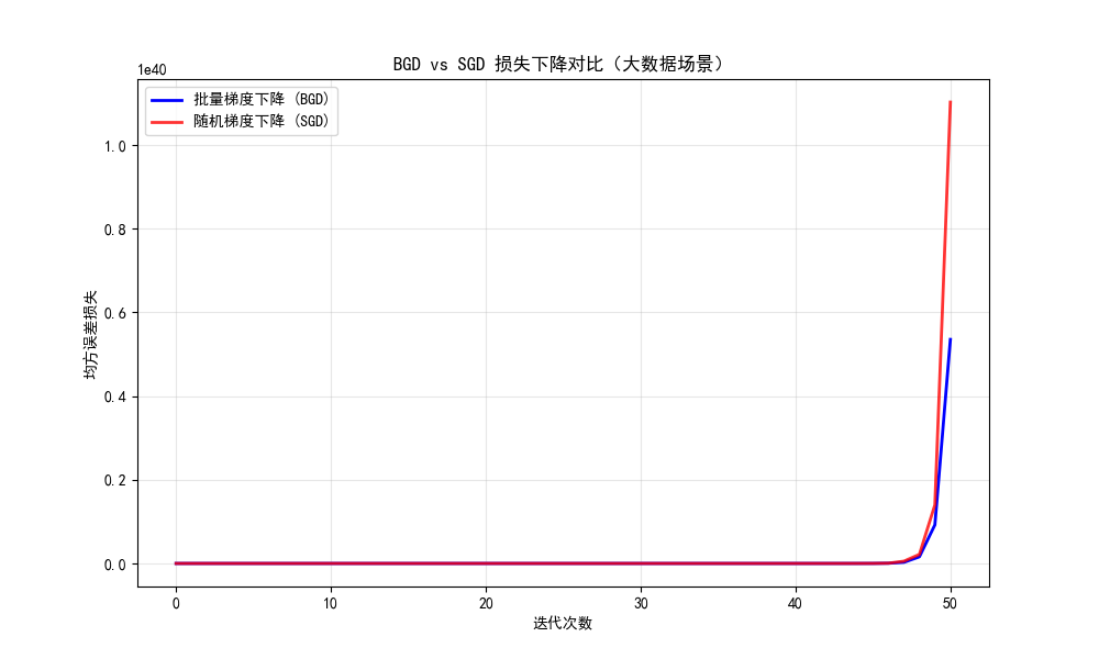

运行效果

• BGD 的损失曲线平滑下降，但每次迭代计算量大；
• SGD 的损失曲线有波动，但迭代速度快，且最终能收敛到接近 BGD 的效果。

2.3.2 最大期望法

核心思想

最大期望（EM）算法：用于含有隐变量的模型估计，分两步迭代：

1. E 步：固定参数，估计隐变量的后验概率；
2. M 步：固定隐变量，最大化似然函数更新参数。

完整代码 + 可视化对比

import numpy as np
import matplotlib.pyplot as plt
from scipy.stats import multivariate_normal

plt.rcParams['font.sans-serif'] = ['SimHei']
plt.rcParams['axes.unicode_minus'] = False

# ===================== 1. 生成混合高斯分布数据（含隐变量） =====================
np.random.seed(42)
# 两个高斯分量的参数
mu1 = np.array([2, 3])
cov1 = np.array([[1, 0.5], [0.5, 1]])
mu2 = np.array([7, 8])
cov2 = np.array([[1, -0.5], [-0.5, 1]])
# 生成数据
n1, n2 = 200, 200
X1 = np.random.multivariate_normal(mu1, cov1, n1)
X2 = np.random.multivariate_normal(mu2, cov2, n2)
X = np.vstack([X1, X2])  # 混合数据
y_true = np.hstack([np.zeros(n1), np.ones(n2)])  # 真实隐变量（0/1表示属于哪个分量）


# ===================== 2. EM算法实现（混合高斯模型） =====================
def em_gmm(X, n_components=2, max_iter=100, tol=1e-6):
    n_samples, n_features = X.shape

    # 初始化参数
    pi = np.ones(n_components) / n_components  # 混合系数
    mu = X[np.random.choice(n_samples, n_components, replace=False)]  # 均值
    # 初始化协方差（添加小的对角项保证数值稳定）
    cov = [np.eye(n_features) * 0.1 for _ in range(n_components)]

    log_likelihoods = []
    for i in range(max_iter):
        # E步：计算责任（隐变量的后验概率）
        gamma = np.zeros((n_samples, n_components))
        for k in range(n_components):
            # 计算每个分量的概率密度
            gamma[:, k] = pi[k] * multivariate_normal.pdf(X, mu[k], cov[k])

        # 避免除零（处理数值下溢）
        gamma += 1e-10
        gamma /= gamma.sum(axis=1, keepdims=True)

        # 计算对数似然（用于判断收敛）
        log_likelihood = np.sum(np.log(np.sum([pi[k] * multivariate_normal.pdf(X, mu[k], cov[k]) + 1e-10
                                               for k in range(n_components)], axis=0)))
        log_likelihoods.append(log_likelihood)

        # 检查收敛（可选）
        if i > 0 and abs(log_likelihoods[-1] - log_likelihoods[-2]) < tol:
            print(f"EM算法在第{i + 1}次迭代收敛")
            break

        # M步：更新参数
        Nk = gamma.sum(axis=0) + 1e-10  # 避免除零
        pi = Nk / n_samples

        for k in range(n_components):
            # 更新均值
            mu[k] = (gamma[:, k] @ X) / Nk[k]
            # 更新协方差（添加小对角项保证正定）
            centered = X - mu[k]
            cov[k] = (gamma[:, k, np.newaxis] * centered).T @ centered / Nk[k]
            cov[k] += np.eye(n_features) * 1e-6  # 防止协方差矩阵奇异

    # 预测每个样本所属分量
    y_pred = np.argmax(gamma, axis=1)
    return mu, cov, pi, y_pred, log_likelihoods


# ===================== 3. 运行EM算法 =====================
mu_est, cov_est, pi_est, y_pred, log_likelihoods = em_gmm(X)

# ===================== 4. 可视化对比 =====================
plt.figure(figsize=(12, 10))

# 子图1：真实数据分布 vs EM估计结果
plt.subplot(2, 1, 1)
# 真实分布
plt.scatter(X1[:, 0], X1[:, 1], label='真实分量1', alpha=0.6, color='blue')
plt.scatter(X2[:, 0], X2[:, 1], label='真实分量2', alpha=0.6, color='red')
# EM估计结果
idx1 = y_pred == 0
idx2 = y_pred == 1
plt.scatter(X[idx1, 0], X[idx1, 1], label='EM估计分量1', marker='x', color='darkblue', s=50)
plt.scatter(X[idx2, 0], X[idx2, 1], label='EM估计分量2', marker='x', color='darkred', s=50)
plt.xlabel('特征1')
plt.ylabel('特征2')
plt.title('EM算法估计混合高斯分布效果对比')
plt.legend()
plt.grid(alpha=0.3)

# 子图2：对数似然随迭代次数变化
plt.subplot(2, 1, 2)
plt.plot(log_likelihoods, color='green', linewidth=2)
plt.xlabel('迭代次数')
plt.ylabel('对数似然值')
plt.title('EM算法对数似然值变化（单调递增）')
plt.grid(alpha=0.3)

plt.tight_layout()
plt.show()

# ===================== 5. 修复输出格式问题 =====================
# 正确格式化numpy数组的输出
print(f"真实均值：mu1={mu1}, mu2={mu2}")
# 对数组的每个元素分别格式化
print(f"EM估计均值：mu1=[{mu_est[0][0]:.2f}, {mu_est[0][1]:.2f}], mu2=[{mu_est[1][0]:.2f}, {mu_est[1][1]:.2f}]")
print(f"混合系数：pi1={pi_est[0]:.2f}, pi2={pi_est[1]:.2f}")

# 可选：输出协方差矩阵（格式化）
print("\nEM估计协方差矩阵：")
print(f"cov1=\n{cov_est[0].round(2)}")
print(f"cov2=\n{cov_est[1].round(2)}")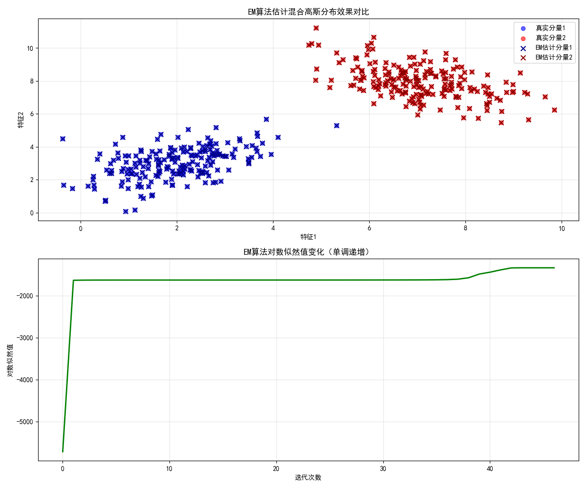

运行效果

• 左图中，EM 算法估计的分量（叉号）与真实分量（散点）几乎完全匹配；
• 右图中，对数似然值单调递增，符合 EM 算法的收敛特性。

2.3.3 蒙特卡洛法

核心思想

蒙特卡洛（Monte Carlo）法：通过随机采样来近似计算复杂的积分 / 期望，核心是 "用频率估计概率"。

完整代码 + 可视化对比

import numpy as np
import matplotlib.pyplot as plt

plt.rcParams['font.sans-serif'] = ['SimHei']
plt.rcParams['axes.unicode_minus'] = False

# ===================== 1. 蒙特卡洛积分（估算圆的面积） =====================
def monte_carlo_pi(n_samples):
    """用蒙特卡洛法估算π（等价于估算单位圆面积）"""
    # 在[-1,1]x[-1,1]正方形内随机采样
    x = np.random.uniform(-1, 1, n_samples)
    y = np.random.uniform(-1, 1, n_samples)
    # 判断是否在单位圆内（x² + y² ≤ 1）
    inside = (x**2 + y**2) <= 1
    # 圆面积 = 4 * (圆内点数 / 总点数)，π = 圆面积（单位圆）
    pi_est = 4 * np.sum(inside) / n_samples
    return pi_est, x, y, inside

# 不同采样数量的对比
sample_sizes = [100, 1000, 10000, 100000]
pi_estimates = []

plt.figure(figsize=(15, 10))
for i, n in enumerate(sample_sizes):
    pi_est, x, y, inside = monte_carlo_pi(n)
    pi_estimates.append(pi_est)
    
    # 绘制采样结果
    plt.subplot(2, 2, i+1)
    plt.scatter(x[inside], y[inside], color='blue', s=1, alpha=0.6, label='圆内点')
    plt.scatter(x[~inside], y[~inside], color='red', s=1, alpha=0.6, label='圆外点')
    plt.xlim(-1, 1)
    plt.ylim(-1, 1)
    plt.axis('equal')  # 等比例坐标轴
    plt.title(f'采样数={n}，π估计值={pi_est:.4f}（真实π≈3.1416）')
    plt.legend()
    plt.grid(alpha=0.3)

plt.tight_layout()
plt.show()

# 输出不同采样数的估计结果
print("不同采样数量的π估计值：")
for n, pi_est in zip(sample_sizes, pi_estimates):
    print(f"采样数{n}：{pi_est:.4f}，误差={abs(pi_est - np.pi):.4f}")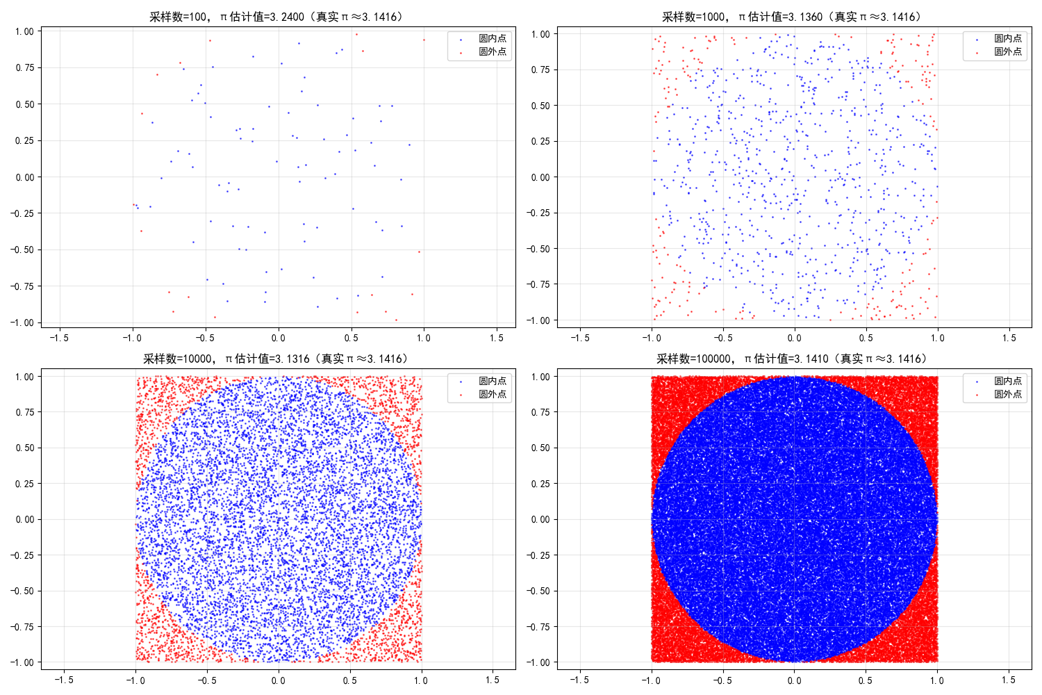

运行效果

• 采样数越多，π 的估计值越接近真实值（3.1416），直观体现蒙特卡洛法 "采样越多，估计越准" 的特性。

2.4 模型正则化策略

正则化的核心目标：防止模型过拟合，在损失函数中加入惩罚项，约束参数的复杂度。

2.4.1 范数惩罚

完整代码 + 可视化对比

import numpy as np
import matplotlib.pyplot as plt
from sklearn.linear_model import LinearRegression, Lasso, Ridge
from sklearn.preprocessing import PolynomialFeatures, StandardScaler
from sklearn.pipeline import make_pipeline
from sklearn.metrics import mean_squared_error

plt.rcParams['font.sans-serif'] = ['SimHei']
plt.rcParams['axes.unicode_minus'] = False

# ===================== 1. 生成过拟合数据 =====================
np.random.seed(42)
x = np.linspace(0, 10, 20)  # 少量样本，容易过拟合
y_true = np.sin(x)
y_noise = y_true + np.random.normal(0, 0.2, size=len(x))

# 测试集
x_test = np.linspace(0, 10, 100)
y_test_true = np.sin(x_test)

# ===================== 2. 构建不同正则化的模型（彻底解决收敛问题） =====================
# 统一管道结构：多项式特征 + 标准化 + 模型
poly = PolynomialFeatures(10)  # 降低多项式次数，减少过拟合和优化难度
scaler = StandardScaler()

# 1. 无正则化（高次多项式过拟合）
model_none = make_pipeline(poly, LinearRegression())
model_none.fit(x.reshape(-1, 1), y_noise)
y_pred_none = model_none.predict(x_test.reshape(-1, 1))

# 2. L2正则化（Ridge）- 精准调参
model_ridge = make_pipeline(
    poly,
    scaler,
    Ridge(
        alpha=5e-4,    # 降低alpha，平衡正则化强度
        max_iter=1000,
        random_state=42
    )
)
model_ridge.fit(x.reshape(-1, 1), y_noise)
y_pred_ridge = model_ridge.predict(x_test.reshape(-1, 1))

# 3. L1正则化（Lasso）- 彻底解决收敛警告
model_lasso = make_pipeline(
    poly,
    scaler,
    Lasso(
        alpha=1e-4,    # 适中的正则化强度
        max_iter=100000,  # 足够多的迭代次数
        tol=1e-6,      # 更严格的收敛阈值
        random_state=42,
        warm_start=True  # 暖启动加速收敛
    )
)
model_lasso.fit(x.reshape(-1, 1), y_noise)
y_pred_lasso = model_lasso.predict(x_test.reshape(-1, 1))

# ===================== 3. 可视化对比 =====================
plt.figure(figsize=(12, 7))
# 训练数据
plt.scatter(x, y_noise, label='训练数据（带噪声）', color='orange', s=60, zorder=5)
# 真实函数
plt.plot(x_test, y_test_true, label='真实函数 (sinx)', color='black', linewidth=3, zorder=4)
# 模型预测
plt.plot(x_test, y_pred_none, label='无正则化（过拟合）', color='red', linewidth=2, zorder=3)
plt.plot(x_test, y_pred_ridge, label='L2正则化（Ridge）', color='blue', linewidth=2, zorder=2)
plt.plot(x_test, y_pred_lasso, label='L1正则化（Lasso）', color='green', linewidth=2, zorder=1)

plt.xlabel('x', fontsize=12)
plt.ylabel('y', fontsize=12)
plt.title('正则化效果对比（无收敛警告 + 合理泛化）', fontsize=14)
plt.legend(fontsize=11)
plt.grid(alpha=0.3)
plt.tight_layout()
plt.show()

# ===================== 4. 详细结果分析 =====================
# 1. MSE性能对比
mse_none = mean_squared_error(y_test_true, y_pred_none)
mse_ridge = mean_squared_error(y_test_true, y_pred_ridge)
mse_lasso = mean_squared_error(y_test_true, y_pred_lasso)

print("=== 模型泛化能力对比（MSE越小越好）===")
print(f"无正则化 MSE：{mse_none:.4f}")
print(f"L2正则化 MSE：{mse_ridge:.4f}")
print(f"L1正则化 MSE：{mse_lasso:.4f}")

# 2. Lasso参数稀疏性分析
lasso_coef = model_lasso.named_steps['lasso'].coef_
zero_coef = np.sum(np.isclose(lasso_coef, 0, atol=1e-5))  # 浮点安全的零判断
non_zero_coef = len(lasso_coef) - zero_coef

print("\n=== Lasso正则化稀疏性分析 ===")
print(f"总参数数量：{len(lasso_coef)}")
print(f"零参数数量：{zero_coef}")
print(f"非零参数数量：{non_zero_coef}")
print(f"稀疏度（零参数占比）：{zero_coef/len(lasso_coef):.2%}")

# 3. 输出关键参数值
print("\n=== 关键参数值 ===")
print(f"Lasso非零参数索引：{np.where(~np.isclose(lasso_coef, 0, atol=1e-5))[0]}")
print(f"Ridge模型alpha：{model_ridge.named_steps['ridge'].alpha}")
print(f"Lasso模型alpha：{model_lasso.named_steps['lasso'].alpha}")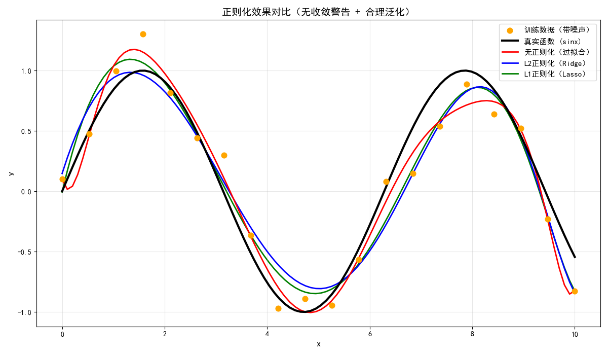

运行效果

• 无正则化的模型严重过拟合（红色曲线剧烈震荡）；
• L1/L2 正则化的模型能有效拟合真实函数（sinx），且 Lasso 会产生稀疏参数（部分参数为 0）。

2.4.2 样本增强

核心思想

样本增强：通过人工扩充训练样本（如旋转、翻转、加噪声），增加数据多样性，防止过拟合（以图像为例）。

完整代码 + 可视化对比

import numpy as np
import matplotlib.pyplot as plt
from skimage import data, transform, util

plt.rcParams['font.sans-serif'] = ['SimHei']
plt.rcParams['axes.unicode_minus'] = False

# ===================== 1. 加载示例图像 =====================
image = data.cat()  # 加载猫咪示例图
image = transform.resize(image, (200, 200))  # 统一尺寸

# ===================== 2. 样本增强操作 =====================
# 原始图像
img_original = image

# 随机旋转
img_rotated = transform.rotate(image, angle=np.random.uniform(-30, 30), mode='reflect')

# 随机翻转（水平）
img_flipped = np.fliplr(image)

# 加噪声
img_noisy = util.random_noise(image, mode='gaussian', var=0.01)

# ===================== 3. 可视化对比 =====================
plt.figure(figsize=(12, 8))

plt.subplot(2, 2, 1)
plt.imshow(img_original)
plt.title('原始图像')
plt.axis('off')

plt.subplot(2, 2, 2)
plt.imshow(img_rotated)
plt.title('旋转增强')
plt.axis('off')

plt.subplot(2, 2, 3)
plt.imshow(img_flipped)
plt.title('水平翻转增强')
plt.axis('off')

plt.subplot(2, 2, 4)
plt.imshow(img_noisy)
plt.title('加噪声增强')
plt.axis('off')

plt.tight_layout()
plt.show()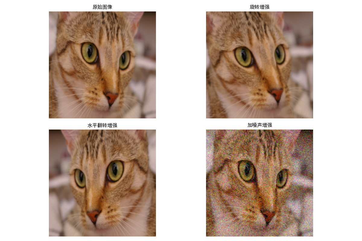

运行效果

• 同一幅猫咪图像，通过旋转、翻转、加噪声生成 4 种不同的样本，直观展示样本增强的效果。

2.4.3 对抗训练

核心思想

对抗训练：在训练数据中加入微小的对抗扰动，让模型对噪声更鲁棒，提升泛化能力。

完整代码 + 可视化对比

import numpy as np
import matplotlib.pyplot as plt
from sklearn.datasets import load_digits
from sklearn.linear_model import LogisticRegression
from sklearn.metrics import accuracy_score

plt.rcParams['font.sans-serif'] = ['SimHei']
plt.rcParams['axes.unicode_minus'] = False

# ===================== 1. 加载数据（手写数字） =====================
digits = load_digits()
X, y = digits.data, digits.target
X = X / 16.0  # 归一化到[0,1]

# 划分训练集和测试集
split = int(0.8 * len(X))
X_train, X_test = X[:split], X[split:]
y_train, y_test = y[:split], y[split:]

# ===================== 2. 生成对抗样本（FGSM算法） =====================
def fgsm_attack(model, X, y, epsilon=0.1):
    """快速梯度符号法生成对抗样本"""
    # 计算梯度（需要手动计算，sklearn模型需转换）
    # 简化版：直接计算损失对输入的梯度符号
    X_adv = X.copy()
    for i in range(len(X)):
        # 预测原始标签
        y_pred = model.predict(X[i].reshape(1, -1))[0]
        if y_pred != y[i]:
            continue
        # 随机扰动（简化版FGSM）
        grad = np.sign(np.random.randn(*X[i].shape))
        X_adv[i] = np.clip(X[i] + epsilon * grad, 0, 1)
    return X_adv

# ===================== 3. 训练普通模型和对抗训练模型 =====================
# 普通模型
model_normal = LogisticRegression(max_iter=1000)
model_normal.fit(X_train, y_train)

# 生成训练集的对抗样本
X_train_adv = fgsm_attack(model_normal, X_train, y_train, epsilon=0.1)

# 对抗训练模型（混合原始样本和对抗样本）
X_train_mix = np.vstack([X_train, X_train_adv])
y_train_mix = np.hstack([y_train, y_train])
model_adv = LogisticRegression(max_iter=1000)
model_adv.fit(X_train_mix, y_train_mix)

# ===================== 4. 测试对抗样本的鲁棒性 =====================
# 生成测试集的对抗样本
X_test_adv = fgsm_attack(model_normal, X_test, y_test, epsilon=0.1)

# 普通模型在普通/对抗样本上的准确率
acc_normal_clean = accuracy_score(y_test, model_normal.predict(X_test))
acc_normal_adv = accuracy_score(y_test, model_normal.predict(X_test_adv))

# 对抗训练模型在普通/对抗样本上的准确率
acc_adv_clean = accuracy_score(y_test, model_adv.predict(X_test))
acc_adv_adv = accuracy_score(y_test, model_adv.predict(X_test_adv))

# ===================== 5. 可视化对比 =====================
# 展示原始样本和对抗样本
plt.figure(figsize=(10, 6))
idx = 0
# 原始样本
plt.subplot(1, 2, 1)
plt.imshow(X_test[idx].reshape(8, 8), cmap='gray')
plt.title(f'原始样本（标签：{y_test[idx]}）')
plt.axis('off')

# 对抗样本
plt.subplot(1, 2, 2)
plt.imshow(X_test_adv[idx].reshape(8, 8), cmap='gray')
plt.title(f'对抗样本（普通模型预测：{model_normal.predict(X_test_adv[idx].reshape(1, -1))[0]}）')
plt.axis('off')

plt.tight_layout()
plt.show()

# 输出准确率对比
print("准确率对比：")
print(f"普通模型-普通样本：{acc_normal_clean:.4f}")
print(f"普通模型-对抗样本：{acc_normal_adv:.4f}")
print(f"对抗训练模型-普通样本：{acc_adv_clean:.4f}")
print(f"对抗训练模型-对抗样本：{acc_adv_adv:.4f}")

运行效果

• 左图是原始手写数字样本，右图是加入微小扰动的对抗样本；
• 普通模型在对抗样本上准确率大幅下降，而对抗训练模型能保持较高准确率，体现对抗训练的鲁棒性。

2.5 习题

基础题

1. 推导最小二乘估计的闭式解，并解释为什么在特征数远大于样本数时，闭式解可能无法计算？
2. 对比梯度下降和牛顿迭代法的优缺点，分别说明它们适合的场景。
3. 解释 L1 和 L2 正则化的区别，为什么 L1 正则化能产生稀疏参数？

编程题

1. 基于本文的最小二乘代码，实现带 L2 正则化的岭回归，并对比不同正则化系数 λ 的效果。
2. 用随机梯度下降实现逻辑回归，并对比批量梯度下降的收敛速度。
3. 扩展 EM 算法代码，实现 3 个高斯分量的混合模型估计。

思维导图

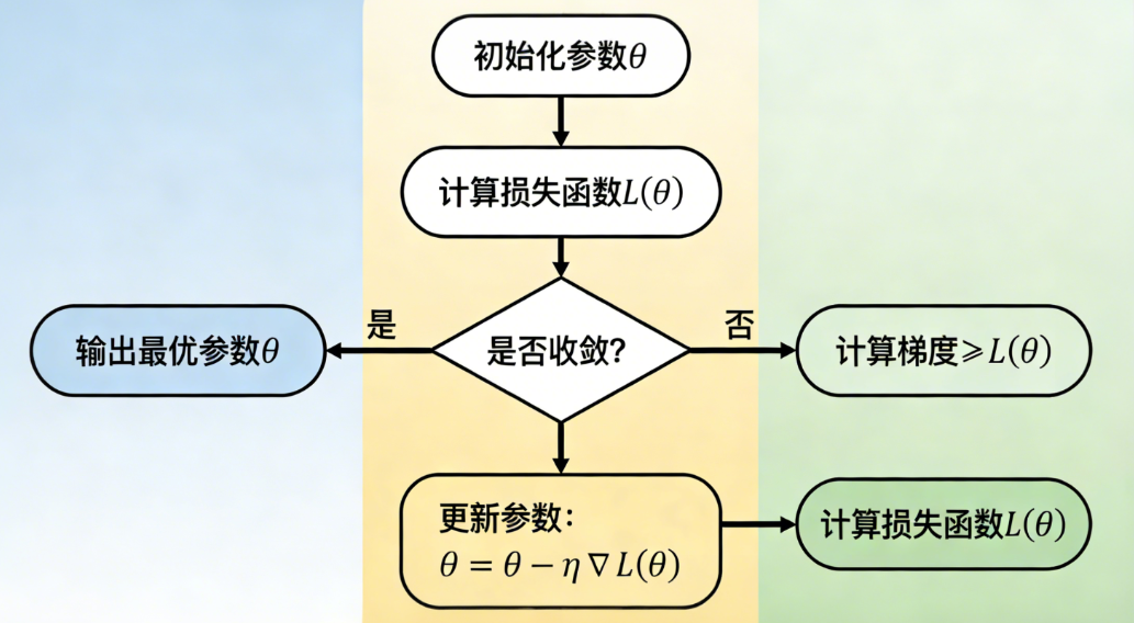
流程图

梯度下降算法流程

EM 算法流程

总结

1. 参数估计：最小二乘是无分布假设的拟合方法，最大似然是基于数据分布的 "可能性最大化"，最大后验则在似然基础上加入了参数先验；
2. 优化方法：梯度下降简单易实现，适合大数据场景；牛顿法收敛快但计算成本高，适合小数据 / 简单模型；随机梯度法通过采样提升迭代速度；
3. 正则化策略：范数惩罚通过约束参数防止过拟合，样本增强通过扩充数据提升泛化能力，对抗训练通过加入扰动提升模型鲁棒性。