目录
一、实验目的
- 掌握卷积神经网络(CNN)的设计与实现:学习并实践如何使用PyTorch框架从零开始构建一个用于图像分类的卷积神经网络模型。
- 理解深度学习模型训练的全过程:深入体验从数据加载与增强、模型定义、设置损失函数与优化器,到执行训练、验证、测试以及使用TensorBoard进行可视化监控的完整流程。
- 学习模型的性能评估方法:掌握除准确率外的多种评估指标,如精确率(Precision)、召回率(Recall)、F1分数(F1-Score),并学会使用混淆矩阵(ConfusionMatrix)对模型分类结果进行深入分析。
- 实现模型的实际部署与应用:将训练好的模型与OpenCV计算机视觉库相结合,开发一个能够调用摄像头、实时检测和识别视野中手写数字的应用程序,实现从理论到实践的跨越。
二、实验内容
- 模型训练(handdemo1.py)
- 数据集:使用经典的手写数字数据集MNIST。脚本通过datasets.ImageFolder从本地路径加载数据,并将其划分为80%的训练集和20%的验证集。
- 数据预处理与增强:对输入的图像进行一系列变换,包括转为单通道灰度图、施加随机旋转(±10度)以增强模型泛化能力、转换为张量(Tensor),并进行归一化处理。
- 模型构建:搭建一个自定义的卷积神经网络CNNNetwork,用于从28x28的数字图像中提取特征并进行分类。
- 训练与评估:模型共训练10个周期(Epochs)。训练过程中,使用Adam优化器和StepLR学习率调度器。每个周期结束后,在验证集上评估模型性能,并保存验证准确率最高的模型。训练的全过程通过TensorBoard进行记录和可视化。
- 最终测试:训练结束后,在测试集上进行最终评估,计算准确率、精确率、召回率、F1分数,并生成混淆矩阵以分析具体类别的分类情况。同时,脚本还会保存被错误分类的样本图片,以供后续分析。
- 实时识别应用(handdemo2.py)
- 模型加载:加载在第一部分中训练并保存的最佳模型文件best_model.pth。
- 实时视频处理 :
- 使用OpenCV启动并读取摄像头视频流。
- 对每一帧图像,通过一个预处理流程(灰度化->高斯模糊->自适应阈值化)将其转换为二值图像,以凸显数字并抑制背景噪声。
- 在二值图像上查找轮廓,并通过尺寸和面积筛选出可能是数字的区域。
-
- 数字识别与可视化 :
- 对每个筛选出的数字轮廓区域进行裁剪,并调整至模型输入的28x28尺寸。
- 将处理后的图像送入加载的CNN模型进行推理,得到预测的数字和置信度。
- 在原始视频帧中,用矩形框标出检测到的数字,并在框上方显示预测结果和置信度,实现实时交互。
- 数字识别与可视化 :
三、实验方法
- 模型架构(CNNNetwork) 该模型是一个小而有效的CNN,其结构如下:
- 输入层:接收1x28x28的单通道灰度图像。
- 卷积层1:使用32个3x3的卷积核,后接批量归一化(BatchNorm)和ReLU激活函数。
- 卷积层2:使用64个3x3的卷积核,同样后接批量归一化和ReLU激活函数。
- 池化层:一个2x2的最大池化层,用于降维和提取关键特征。
- 正则化:一个Dropout层,以50%的概率随机丢弃神经元,有效防止过拟合。
- 全连接层:经过展平(Flatten)操作后,连接两个全连接层。第一个全连接层有128个神经元,并带有批量归一化和ReLU激活;第二个是输出层,有10个神经元,分别对应0-9十个数字的得分。
- 训练策略
- 损失函数:采用nn.CrossEntropyLoss,这是多分类任务的标准选择。
- 优化器:使用optim.Adam,学习率为0.001,它是一种高效且收敛速度快的优化算法。
- 学习率调度:使用StepLR调度器,每隔5个周期将学习率乘以0.1,有助于在训练后期更精细地调整权重,寻找最优解。
- 实时数字分割方法 在handdemo2.py中,数字的实时检测与分割依赖于一套经典的OpenCV处理流程:
- 预处理:preprocess_image函数通过高斯模糊和自适应阈值,从复杂的摄像头背景中提取出清晰的二值化前景(即数字)。
- **轮廓发现:**find_digit_contours函数在二值图像上寻找所有独立的白色区域轮廓。
- **轮廓筛选:**通过设定合理的宽度、高度和面积阈值,过滤掉由噪声或非数字物体产生的过小或过大的轮廓,最终分离出独立的数字区域。
四、算法特色
- 全面的训练监控与评估此项目的一大特色是其详尽的训练监控和评估体系。不仅使用了TensorBoard实时追踪损失、准确率、学习率等关键指标,还在训练结束后计算了精确率、召回率、F1分数等多维度指标,并绘制了混淆矩阵。这种全面的分析远比单一的准确率更能揭示模型的真实性能和潜在问题。
- 稳健的模型设计 模型CNNNetwork中同时包含了批量归一化(BatchNormalization) 和Dropout。前者可以加速模型收敛,使训练过程更稳定;后者则是一种强大的正则化手段,有效降低了模型过拟合的风险。
- 完整的端到端系统本实验没有止步于训练出一个模型文件,而是进一步通过handdemo2.py将其封装成一个实用的实时应用。这展示了从数据到模型,再到应用的完整深度学习项目流程,具有很高的实践价值。
- 经典CV与深度学习的融合在实时应用中,项目巧妙地融合了传统计算机视觉(OpenCV)与深度学习(PyTorch)。利用OpenCV成熟的图像处理技术(如阈值化、轮廓检测)来完成前景分割这一"粗活",然后将分割出的、标准化的数字图像交给深度学习模型完成最关键的分类"细活",是解决此类问题的经典高效范式。
五、实验结果及分析
实验源代码:
python
handdemo1
import time
import torch
from torch import nn, optim
from torchvision import transforms, datasets
from torch.utils.data import DataLoader, random_split
from torch.optim.lr_scheduler import StepLR
from torch.utils.tensorboard import SummaryWriter
from pathlib import Path
from sklearn.metrics import confusion_matrix, precision_score, recall_score, f1_score
import seaborn as sns
import matplotlib.pyplot as plt

# 定义卷积神经网络
class CNNNetwork(nn.Module):
    def __init__(self):
        super().__init__()
        self.conv1 = nn.Conv2d(1, 32, kernel_size=3, padding=1)  # 输入通道为1,输出通道为32
        self.bn1 = nn.BatchNorm2d(32)  # 批量归一化
        self.conv2 = nn.Conv2d(32, 64, kernel_size=3, padding=1)  # 输入通道为32,输出通道为64
        self.bn2 = nn.BatchNorm2d(64)  # 批量归一化
        self.dropout = nn.Dropout(0.5)  # Dropout
        self.fc1 = nn.Linear(self._get_flatten_size((1, 28, 28)), 128)  # 动态计算全连接层输入尺寸
        self.bn3 = nn.BatchNorm1d(128)  # 批量归一化
        self.fc2 = nn.Linear(128, 10)  # 输出层

    def _get_flatten_size(self, input_shape):
        x = torch.zeros(1, *input_shape)
        x = self.conv1(x)
        x = self.conv2(x)
        x = torch.max_pool2d(x, 2)
        return x.numel()

    def forward(self, x):
        x = torch.relu(self.bn1(self.conv1(x)))
        x = torch.relu(self.bn2(self.conv2(x)))
        x = torch.max_pool2d(x, 2)  # 池化层
        x = self.dropout(x)
        x = x.view(x.size(0), -1)  # 展平
        x = torch.relu(self.bn3(self.fc1(x)))
        x = self.fc2(x)
        return x

if __name__ == '__main__':
    # 设置设备
    device = torch.device("cuda" if torch.cuda.is_available() else "cpu")
    # 数据增强与预处理
    transform = transforms.Compose([
        transforms.Grayscale(num_output_channels=1),
        transforms.RandomRotation(10),  # 随机旋转
        transforms.ToTensor(),
        transforms.Normalize((0.5,), (0.5,))  # 归一化
    ])
    try:
        dataset = datasets.ImageFolder(root="C:/Users/L1307/Desktop/深度学习/train1", transform=transform)
    except Exception as e:
        print(f"Error loading dataset: {e}")
        exit()
    train_size = int(0.8 * len(dataset))
    val_size = len(dataset) - train_size
    train_dataset, val_dataset = random_split(dataset, [train_size, val_size])

    train_loader = DataLoader(train_dataset, batch_size=64, shuffle=True, num_workers=4)
    val_loader = DataLoader(val_dataset, batch_size=64, shuffle=False, num_workers=4)
    # 加载测试集
    test_dataset = datasets.ImageFolder(root="C:/Users/L1307/Desktop/深度学习/train1", transform=transform)
    test_loader = DataLoader(test_dataset, batch_size=64, shuffle=False, num_workers=4)

    # 初始化模型、损失函数和优化器
    model = CNNNetwork().to(device)
    criterion = nn.CrossEntropyLoss()
    optimizer = optim.Adam(model.parameters(), lr=0.001)
    scheduler = StepLR(optimizer, step_size=5, gamma=0.1)

    # 初始化 TensorBoard
    writer = SummaryWriter(log_dir='C:/Users/L1307/Desktop/深度学习/runs/CNN')

    # 记录模型结构
    dummy_input = torch.randn(1, 1, 28, 28).to(device)
    writer.add_graph(model, dummy_input)

    start_time = time.time()

    # 训练模型
    best_val_accuracy = 0
    for epoch in range(10):
        model.train()
        running_loss = 0.0
        epoch_start_time = time.time()

        for batch_idx, (data, label) in enumerate(train_loader):
            data, label = data.to(device), label.to(device)

            # 前向传播
            output = model(data)
            loss = criterion(output, label)

            # 反向传播与优化
            optimizer.zero_grad()
            loss.backward()
            optimizer.step()

            running_loss += loss.item()

            # 每 10 个 batch 记录一次训练损失
            if batch_idx % 10 == 0:
                writer.add_scalar('Training Loss', loss.item(), epoch * len(train_loader) + batch_idx)

        scheduler.step()
        avg_loss = running_loss / len(train_loader)
        writer.add_scalar('Average Training Loss', avg_loss, epoch)
        writer.add_scalar('Learning Rate', scheduler.get_last_lr()[0], epoch)

        epoch_end_time = time.time()
        epoch_duration = epoch_end_time - epoch_start_time
        writer.add_scalar('Epoch Training Time (s)', epoch_duration, epoch)

        print(f"Epoch {epoch + 1}, Loss: {avg_loss:.4f}, LR: {scheduler.get_last_lr()[0]:.6f}, Time: {epoch_duration:.2f}s")

        # 验证模型
        model.eval()
        val_loss = 0.0
        val_correct = 0
        with torch.no_grad():
            for data, label in val_loader:
                data, label = data.to(device), label.to(device)
                output = model(data)
                loss = criterion(output, label)
                val_loss += loss.item()
                val_correct += (output.argmax(1) == label).sum().item()

        val_accuracy = val_correct / len(val_dataset)
        writer.add_scalar('Validation Loss', val_loss / len(val_loader), epoch)
        writer.add_scalar('Validation Accuracy', val_accuracy, epoch)
        print(f"Validation Loss: {val_loss / len(val_loader):.4f}, Accuracy: {val_accuracy:.4f}")

        # 保存最优模型
        if val_accuracy > best_val_accuracy:
            best_val_accuracy = val_accuracy
            torch.save(model.state_dict(), 'C:/Users/L1307/Desktop/深度学习/runs/CNN/best_model.pth')

    end_time = time.time()
    total_duration = end_time - start_time
    print(f"Total training time: {total_duration:.2f}s")

    # 测试模型
    model.eval()
    correct = 0
    total = 0
    wrong_samples_path = Path('C:/Users/L1307/Desktop/深度学习/runs/CNN/wrong_samples')
    wrong_samples_path.mkdir(exist_ok=True)
    all_preds = []
    all_labels = []
    with torch.no_grad():
        for data, label in test_loader:
            data, label = data.to(device), label.to(device)
            output = model(data)
            _, predicted = torch.max(output, 1)
            correct += (predicted == label).sum().item()
            total += label.size(0)

            all_preds.extend(predicted.cpu().numpy())
            all_labels.extend(label.cpu().numpy())
            # Save misclassified samples
            for i in range(data.size(0)):
                if predicted[i] != label[i]:
                    img = data[i].cpu().squeeze(0) * 0.5 + 0.5  # 去归一化
                    img_pil = transforms.ToPILImage()(img)
                    wrong_img_path = wrong_samples_path / f"wrong_pred_{predicted[i].item()}_true_{label[i].item()}.png"
                    img_pil.save(wrong_img_path)

    # 计算测试集评估指标
    accuracy = correct / total
    precision = precision_score(all_labels, all_preds, average='macro')
    recall = recall_score(all_labels, all_preds, average='macro')
    f1 = f1_score(all_labels, all_preds, average='macro')
    writer.add_scalar('Test Accuracy', accuracy, 0)
    writer.add_scalar('Test Precision', precision, 0)
    writer.add_scalar('Test Recall', recall, 0)
    writer.add_scalar('Test F1 Score', f1, 0)

    print(f"Test Accuracy: {accuracy:.4f}")
    print(f"Test Precision: {precision:.4f}, Recall: {recall:.4f}, F1 Score: {f1:.4f}")

    # 绘制并记录混淆矩阵
    cm = confusion_matrix(all_labels, all_preds)
    plt.figure(figsize=(10, 8))
    sns.heatmap(cm, annot=True, fmt='d', cmap='Blues', xticklabels=test_dataset.classes, yticklabels=test_dataset.classes)
    plt.ylabel('Actual')
    plt.xlabel('Predicted')
    plt.title('Confusion Matrix')
    writer.add_figure('Confusion Matrix', plt.gcf())

    # 关闭 TensorBoard
    writer.close()
handdemo2
import torch
import torch.nn as nn
import cv2
from torchvision import transforms
from PIL import Image

# 定义CNN网络结构
class CNNNetwork(nn.Module):
    def __init__(self):
        super().__init__()
        self.conv1 = nn.Conv2d(1, 32, kernel_size=3, padding=1)  # 输入通道1,输出通道32
        self.bn1 = nn.BatchNorm2d(32)  # 批归一化
        self.conv2 = nn.Conv2d(32, 64, kernel_size=3, padding=1)  # 输入通道32,输出通道64
        self.bn2 = nn.BatchNorm2d(64)  # 批归一化
        self.dropout = nn.Dropout(0.5)  # Dropout
        self.fc1 = nn.Linear(self._get_flatten_size((1, 28, 28)), 128)  # 动态计算全连接层的输入大小
        self.bn3 = nn.BatchNorm1d(128)  # 批归一化
        self.fc2 = nn.Linear(128, 10)  # 输出层

    def _get_flatten_size(self, input_shape):
        x = torch.zeros(1, *input_shape)
        x = self.conv1(x)
        x = self.conv2(x)
        x = torch.max_pool2d(x, 2)
        return x.numel()

    def forward(self, x):
        x = torch.relu(self.bn1(self.conv1(x)))
        x = torch.relu(self.bn2(self.conv2(x)))
        x = torch.max_pool2d(x, 2)  # 池化层
        x = self.dropout(x)
        x = x.view(x.size(0), -1)  # 展平
        x = torch.relu(self.bn3(self.fc1(x)))
        x = self.fc2(x)
        return x
# 图像预处理函数
def preprocess_image(image):
    # 转为灰度图
    gray = cv2.cvtColor(image, cv2.COLOR_BGR2GRAY)
    # 高斯模糊减少噪声
    blurred = cv2.GaussianBlur(gray, (5, 5), 0)
    # 自适应阈值处理
    thresh = cv2.adaptiveThreshold(blurred, 255, cv2.ADAPTIVE_THRESH_GAUSSIAN_C,cv2.THRESH_BINARY_INV, 11, 2)
    return thresh


# 查找和提取数字轮廓
def find_digit_contours(binary_image):
    # 查找轮廓
    contours, _ = cv2.findContours(binary_image.copy(), cv2.RETR_EXTERNAL, cv2.CHAIN_APPROX_SIMPLE)
    # 过滤有效的数字轮廓
    digit_contours = []
    for contour in contours:
        # 获取轮廓的外接矩形
        x, y, w, h = cv2.boundingRect(contour)
        # 过滤掉过小的区域
        if w > 20 and h > 20 and w < 300 and h < 300:
            # 计算轮廓的面积
            area = cv2.contourArea(contour)
            # 过滤掉过小的面积轮廓
            if area > 100:
                digit_contours.append((x, y, w, h))
    return digit_contours

# 加载训练好的模型
def load_model(model_path):
    device = torch.device("cuda" if torch.cuda.is_available() else "cpu")
    model = CNNNetwork().to(device)
    try:
        model.load_state_dict(torch.load(model_path, map_location=device))
        print(f"Model loaded successfully: {model_path}")
    except Exception as e:
        print(f"Error loading model: {e}")
        raise

    model.eval()
    return model, device

# 识别数字
def recognize_digit(model, device, digit_image):
    # 将图像调整为28x28大小
    resized_digit = cv2.resize(digit_image, (28, 28))
    # 转为PIL图像
    pil_image = Image.fromarray(resized_digit)
    # 使用与训练时相同的预处理
    transform = transforms.Compose([transforms.ToTensor(), transforms.Normalize((0.5,), (0.5,))])
    # 转为tensor
    tensor = transform(pil_image).unsqueeze(0).to(device)
    # 预测
    with torch.no_grad():
        output = model(tensor)
        _, predicted = torch.max(output, 1)
        confidence = torch.nn.functional.softmax(output, dim=1)[0, predicted.item()].item()
    return predicted.item(), confidence

# 主函数
def main():
    # 模型路径
    model_path = "C:/Users/L1307/Desktop/deep learning/runs/CNN/best_model.pth"
    # 加载模型
    try:
        model, device = load_model(model_path)
    except Exception as e:
        print(f"Unable to load model: {e}")
        return
    # 打开摄像头
    cap = cv2.VideoCapture(0)
    # 检查摄像头是否打开成功
    if not cap.isOpened():
        print("Error: Could not open camera.")
        return
    print("Camera opened, start recognizing digits...")
    print("Press 'q' to exit the program")
    canvas_width = 800
    canvas_height = 600
    font = cv2.FONT_HERSHEY_SIMPLEX
    while True:
        # 读取摄像头帧
        ret, frame = cap.read()
        if not ret:
            print("Error: Could not read frame from camera.")
            break
        # 调整帧大小
        frame = cv2.resize(frame, (canvas_width, canvas_height))
        # 预处理图像
        binary_image = preprocess_image(frame)
        # 查找数字轮廓
        digit_contours = find_digit_contours(binary_image)
        # 对每个检测到的区域进行数字识别
        for i, (x, y, w, h) in enumerate(digit_contours):
            # 提取数字区域
            digit_roi = binary_image[y:y + h, x:x + w]
            # 识别数字
            predicted_digit, confidence = recognize_digit(model, device, digit_roi)
            cv2.rectangle(frame, (x, y), (x + w, y + h), (0, 255, 0), 2)
            label = f"{predicted_digit} ({confidence:.2f})"
            cv2.putText(frame, label, (x, y - 10), font, 0.6, (0, 255, 0), 2)
            processed_digit = cv2.resize(digit_roi, (200, 200))
            frame[10:210, 10:210] = cv2.cvtColor(processed_digit, cv2.COLOR_GRAY2BGR)
            label_position = (10, 240)
            label = f"Pred: {predicted_digit}, Conf: {confidence:.2f}"
            cv2.putText(frame, label, label_position, font, 0.6, (0, 255, 0), 2)
        # 显示结果
        cv2.putText(frame, "Press 'q' to exit the program", (300, 30), font, 0.6, (255, 0, 0), 2)
        cv2.imshow("Digit Recognition", frame)
        key = cv2.waitKey(1) & 0xFF
        # 按下 'q' 键退出
        if key == ord('q'):
            break
    # 释放摄像头并关闭窗口
    cap.release()
    cv2.destroyAllWindows()
if __name__ == "__main__":
    main()
模型训练结果

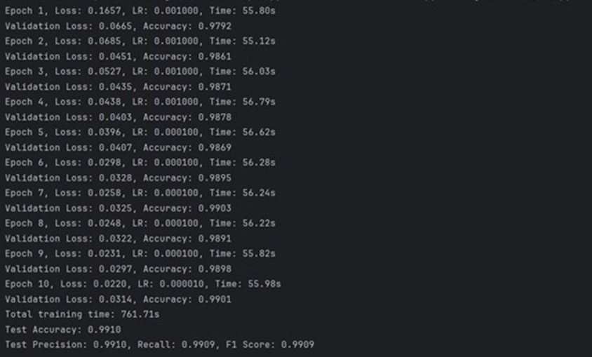
在handdemo1.py的训练过程中,每个周期结束后会输出该周期的训练损失、测试损失、测试准确率和训练时间。典型的输出格式:
测试准确率、精确率、召回率和F1分数均达到了约 99.1% 的极高水平。这表明模型不仅准确率高,而且在各个评估维度上都表现稳健,具有非常强的分类能力和泛化性。从10个周期的训练日志可以看出,验证集准确率(Validation Accuracy)一直保持在97.9%以上,并稳定提升。这说明模型在训练过程中收敛得很好,没有出现明显的过拟合或训练不稳定的情况。
验证模型识别情况:
对于数字"5",模型以 100% 的置信度(Conf: 1.00)准确识别。
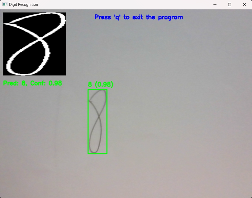
对于数字"8",模型也以 98% 的高置信度(Conf: 0.98)准确识别。