记 N ( t ) N(t) N(t) 为 t t t 时刻染病人数,则 t + △ t t+△t t+△t 时刻的染病人数为 N ( t + △ t ) N(t+△t) N(t+△t)
从 t → t + △ t t→ t+△t t→t+△t 时间内,净增加的染病人数为 N ( t + △ t ) − N ( t ) N(t+△t)-N(t) N(t+△t)−N(t)
有:
N ( t + △ t ) − N ( t ) = λ N ( t ) △ t N(t+△t)-N(t) = \lambda N(t)△t N(t+△t)−N(t)=λN(t)△t
若记 t = 0 t=0 t=0 时刻,染病人数为 N 0 N_0 N0。则由假设2,在上式两端同时除以 △ t △t △t,并令 △ t → 0 △t→0 △t→0,得传染病染病人数的微分方程预测模型:
{ d N ( t ) d t = λ N ( t ) , t > 0 , N ( 0 ) = N 0 . \begin{cases} \dfrac{dN(t)}{dt} = \lambda N(t),\quad t > 0,\\6pt N(0) = N_0. \end{cases} ⎩ ⎨ ⎧dtdN(t)=λN(t),t>0,N(0)=N0.
利用分离变量法可很容易地得到该模型的解析解为:
N ( t ) = N 0 e λ t N(t)=N_0e^{\lambda t} N(t)=N0eλt
每个病人每天可使 λ s ( t ) \lambda s(t) λs(t) 个健康者变为病人,而 t t t 时刻病人总数为 N i ( t ) Ni(t) Ni(t),故在 t → t + △ t t→t+△t t→t+△t 时段
内,共有 λ N s ( t ) i ( t ) △ t \lambda Ns(t)i(t)\triangle t λNs(t)i(t)△t 个健康者被感染
于是有:
N i ( t + Δ t ) − N i ( t ) Δ t = λ N s ( t ) i ( t ) \frac{Ni(t+\Delta t) - Ni(t)}{\Delta t} = \lambda N s(t) i(t) ΔtNi(t+Δt)−Ni(t)=λNs(t)i(t)
令 △ t → 0 \triangle t \rightarrow 0 △t→0, 得微分方程:
d i ( t ) d t = λ s ( t ) i ( t ) \frac{di(t)}{dt} = \lambda s(t) i(t) dtdi(t)=λs(t)i(t)
又由假设(3)知, s ( t ) = 1 − i ( t ) s(t)=1-i(t) s(t)=1−i(t),代入上式得:
d i ( t ) d t = λ i ( t ) ( 1 − i ( t ) ) \frac{di(t)}{dt} = \lambda i(t)(1-i(t)) dtdi(t)=λi(t)(1−i(t))
假定起始时( t = 0 t=0 t=0),病人占总人口的比例为 i ( 0 ) = i 0 i(0)=i_0 i(0)=i0。 于是 SI 模型可描述为:
{ d i ( t ) d t = λ i ( t ) ( 1 − i ( t ) ) , t > 0 i ( 0 ) = i 0 \begin{cases} \dfrac{di(t)}{dt} = \lambda i(t)(1-i(t)),\quad t > 0\\ i(0) = i_0 \end{cases} ⎩ ⎨ ⎧dtdi(t)=λi(t)(1−i(t)),t>0i(0)=i0
用分离变量法求解此微分方程初值问题,得解析解为:
i ( t ) = 1 1 + ( 1 i 0 − 1 ) e − λ t i(t) = \frac{1}{1+\left( \frac{1}{i_0} - 1 \right) e^{-\lambda t}} i(t)=1+(i01−1)e−λt1
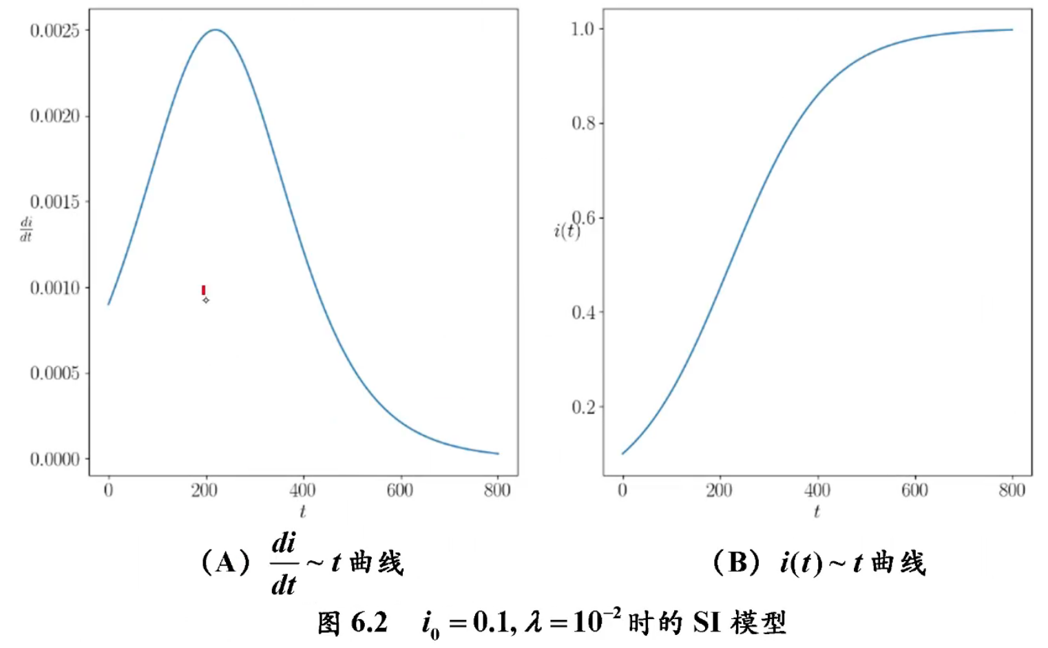
该模型事实上就是 Logistic 模型。病人占总人口的最大比例为 1 1 1,即当 t → ∞ t \to \infty t→∞ 时,区域内所有人都被传染
医学上称 d i d t ∼ t \dfrac{di}{dt} \sim t dtdi∼t 为传染病曲线,它表示传染病人增加率与时间的关系
当病人总量占总人口比值达到 i = 1 2 i=\dfrac{1}{2} i=21时, d i d t \dfrac{di}{dt} dtdi达到最大值,即 d 2 i d t 2 = 0 \dfrac{d^2i}{dt^2}=0 dt2d2i=0,也就是说,此时达到传染病传染高峰期。
传染病高峰到来的时刻为:
t m = 1 λ ln ( 1 i 0 − 1 ) t_m = \frac{1}{\lambda} \ln\left( \frac{1}{i_0} - 1 \right) tm=λ1ln(i01−1)
医学上,这一结果具有重要的意义。由于 t m t_m tm与 λ \lambda λ成反比,故当 λ \lambda λ(反应医疗水平或传染控制措施的有效性)增大时, t m t_m tm将变小,预示着传染病高峰期来得越早。若已知日接触率 λ \lambda λ(由统计数据得出),即可预报传染病高峰到来的时间 t m t_m tm,这对于防治传染病是有益处的。
当 t → ∞ t \to \infty t→∞时, i ( t ) → 1 i(t) \to 1 i(t)→1,即最后人人都要生病。这显然是不符合实际情况的。其原因是假设中未考虑病人得病后可以治愈,人群中的健康者只能变为病人,而病人不会变为健康者。而事实上对某些传染病,如伤风、痢疾等病人治愈后免疫力低下,可假定无免疫性。于是病人被治愈后成为健康者,健康者还可以被感染再变成病人。
3. SIS模型
SIS模型在SI模型假设的基础上,进一步假设:
每天被治愈的病人人数占病人总数的比例为 μ \mu μ
病人被治愈后成为仍可被感染的健康者
于是 SI 模型可被修正为 SIS 模型:
{ d i ( t ) d t = λ i ( t ) ( 1 − i ( t ) ) − μ i ( t ) , t > 0 i ( 0 ) = i 0 \begin{cases} \dfrac{di(t)}{dt} = \lambda i(t)(1-i(t)) - \mu i(t),\quad t > 0 i(0) = i_0 \end{cases} {dtdi(t)=λi(t)(1−i(t))−μi(t),t>0i(0)=i0
利用 σ \sigma σ的定义,方程可改写为:
{ d i d t = − λ i i − ( 1 − 1 σ ) , t > 0 i ( 0 ) = i 0 \begin{cases} \dfrac{di}{dt} = -\lambda i \left i - \\left( 1 - \\dfrac{1}{\\sigma} \\right) \\right,\quad t > 0 \\ i(0) = i_0 \end{cases} ⎩ ⎨ ⎧dtdi=−λii−(1−σ1),t>0i(0)=i0
对所有人群, s ( t ) + i ( t ) + r ( t ) = 1 s(t)+i(t)+r(t)=1 s(t)+i(t)+r(t)=1
对系统移出者r, N d r d t = μ N i N\dfrac{dr}{dt} = \mu N i Ndtdr=μNi
对病人i, N d i d t = λ N s i − μ N i N\dfrac{di}{dt} = \lambda N s i - \mu N i Ndtdi=λNsi−μNi
对健康者s, N d s d t = − λ N s i N\dfrac{ds}{dt} = -\lambda N s i Ndtds=−λNsi
联立得到SIR模型:
{ d i d t = λ s i − μ i d s d t = − λ s i d r d t = μ i i ( 0 ) = i 0 , s ( 0 ) = s 0 , r ( 0 ) = 0 \begin{cases} \dfrac{di}{dt} = \lambda s i - \mu i \\ \dfrac{ds}{dt} = -\lambda s i \\ \dfrac{dr}{dt} = \mu i \\ i(0) = i_0, s(0)=s_0, r(0) = 0 \end{cases} ⎩ ⎨ ⎧dtdi=λsi−μidtds=−λsidtdr=μii(0)=i0,s(0)=s0,r(0)=0
代数形式:
max ( 或 min ) z = c 1 x 1 + c 2 x 2 + ⋯ + c n x n s.t. { a 11 x 1 + a 12 x 2 + ⋯ + a 1 n x n ≤ ( 或 = , ≥ ) b 1 a 21 x 1 + a 22 x 2 + ⋯ + a 2 n x n ≤ ( 或 = , ≥ ) b 2 ⋮ a m 1 x 1 + a m 2 x 2 + ⋯ + a m n x n ≤ ( 或 = , ≥ ) b m x 1 , x 2 , ... , x n ≥ 0 \begin{aligned} &\max\; (\text{或}\;\min)\; z = c_1 x_1 + c_2 x_2 + \dots + c_n x_n \\ \text{s.t.} &\begin{cases} a_{11} x_1 + a_{12} x_2 + \dots + a_{1n} x_n \le (\text{或}=,\;\ge) b_1 \\ a_{21} x_1 + a_{22} x_2 + \dots + a_{2n} x_n \le (\text{或}=,\;\ge) b_2 \\ \quad\quad\quad\quad\quad\quad\quad\vdots \\ a_{m1} x_1 + a_{m2} x_2 + \dots + a_{mn} x_n \le (\text{或}=,\;\ge) b_m \\ x_1, x_2, \dots, x_n \ge 0 \end{cases} \end{aligned} s.t.max(或min)z=c1x1+c2x2+⋯+cnxn⎩ ⎨ ⎧a11x1+a12x2+⋯+a1nxn≤(或=,≥)b1a21x1+a22x2+⋯+a2nxn≤(或=,≥)b2⋮am1x1+am2x2+⋯+amnxn≤(或=,≥)bmx1,x2,...,xn≥0
简写为:
max ( 或 min ) z = ∑ j = 1 n c j x j s.t. { ∑ j = 1 n a i j x j ≤ ( 或 = , ≥ ) b i , i = 1 , 2 , ... , m , x j ≥ 0 , j = 1 , 2 , ... , n \begin{aligned} &\max\; (\text{或}\;\min)\; z = \sum_{j=1}^n c_j x_j \\ \text{s.t.} &\begin{cases} \displaystyle\sum_{j=1}^n a_{ij} x_j \le (\text{或}=,\;\ge) b_i,\quad i=1,2,\dots,m, \\ x_j \ge 0,\quad j=1,2,\dots,n \end{cases} \end{aligned} s.t.max(或min)z=j=1∑ncjxj⎩ ⎨ ⎧j=1∑naijxj≤(或=,≥)bi,i=1,2,...,m,xj≥0,j=1,2,...,n
向量形式为:
max ( 或 min ) z = c T x s.t. { ∑ j = 1 n P j x j ≤ ( 或 = , ≥ ) b x ≥ 0 \begin{aligned} &\max\; (\text{或}\;\min)\; z = \mathbf{c}^T \mathbf{x} \\ \text{s.t.} &\begin{cases} \displaystyle\sum_{j=1}^n \mathbf{P}_j x_j \le (\text{或}=,\;\ge) \mathbf{b} \\ \mathbf{x} \ge \mathbf{0} \end{cases} \end{aligned} s.t.max(或min)z=cTx⎩ ⎨ ⎧j=1∑nPjxj≤(或=,≥)bx≥0
矩阵形式为:
max ( 或 min ) z = c T x s.t. { A x ≤ ( 或 = , ≥ ) b x ≥ 0 \begin{aligned} &\max\; (\text{或}\;\min)\; z = \mathbf{c}^T \mathbf{x} \\ \text{s.t.} &\begin{cases} A\mathbf{x} \le (\text{或}=,\;\ge) \mathbf{b} \\ \mathbf{x} \ge \mathbf{0} \end{cases} \end{aligned} s.t.max(或min)z=cTx{Ax≤(或=,≥)bx≥0
c = c 1 , c 2 , ... , c n T \mathbf{c} = c_1, c_2, \\dots, c_n^T c=c1,c2,...,cnT: 目标函数的系数向量,即价值向量
x = x 1 , x 2 , ... , x n T \mathbf{x} = x_1, x_2, \\dots, x_n^T x=x1,x2,...,xnT: 决策向量
A = ( a i j ) m × n A = (a_{ij})_{m \times n} A=(aij)m×n: 约束方程组的系数矩阵
P j = a 1 j , a 2 j , ... , a m j T , j = 1 , 2 , ... , n \mathbf{P}_j = a_{1j}, a_{2j}, \\dots, a_{mj}^T,\; j=1,2,\dots,n Pj=a1j,a2j,...,amjT,j=1,2,...,n: A A A的列向量, 又称为约束方程组的系数向量
b = b 1 , b 2 , ... , b m T \mathbf{b} = b_1, b_2, \\dots, b_m^T b=b1,b2,...,bmT: 约束方程组的常数向量
可行解 x x x: 满足约束条件的解
最优解 x x x: 使目标函数最大or最小的可行解
可行域 R R R: 所有可行解 x x x构成的集合
求解:
图解法(两个决策变量)
单纯形法(决策变量的数量不多)
MATLAB, Python, LINGO
整数规划
纯整数规划:全部决策变量都必须取整数值的整数规划模型
混合整数规划:决策变量中有一部分必须取整数值,另一部分可以不取整数值的整数规划模型
0-1整数规划:决策变量只能取0或1的整数规划 -> 二值问题
max ( 或 min ) z = ∑ j = 1 n c j x j s.t. { ∑ j = 1 n a i j x j ≤ ( 或 = , ≥ ) b i , i = 1 , 2 , ... , m , x j ≥ 0 , j = 1 , 2 , ... , n x 1 , x 2 , . . . , x n 中部分或全部取整数 \begin{aligned} &\max\; (\text{或}\;\min)\; z = \sum_{j=1}^n c_j x_j \\ \text{s.t.} &\begin{cases} \displaystyle\sum_{j=1}^n a_{ij} x_j \le (\text{或}=,\;\ge) b_i,\quad i=1,2,\dots,m, \\ x_j \ge 0,\quad j=1,2,\dots,n \\ x_1,x_2,...,x_n \text{中部分或全部取整数} \end{cases} \end{aligned} s.t.max(或min)z=j=1∑ncjxj⎩ ⎨ ⎧j=1∑naijxj≤(或=,≥)bi,i=1,2,...,m,xj≥0,j=1,2,...,nx1,x2,...,xn中部分或全部取整数
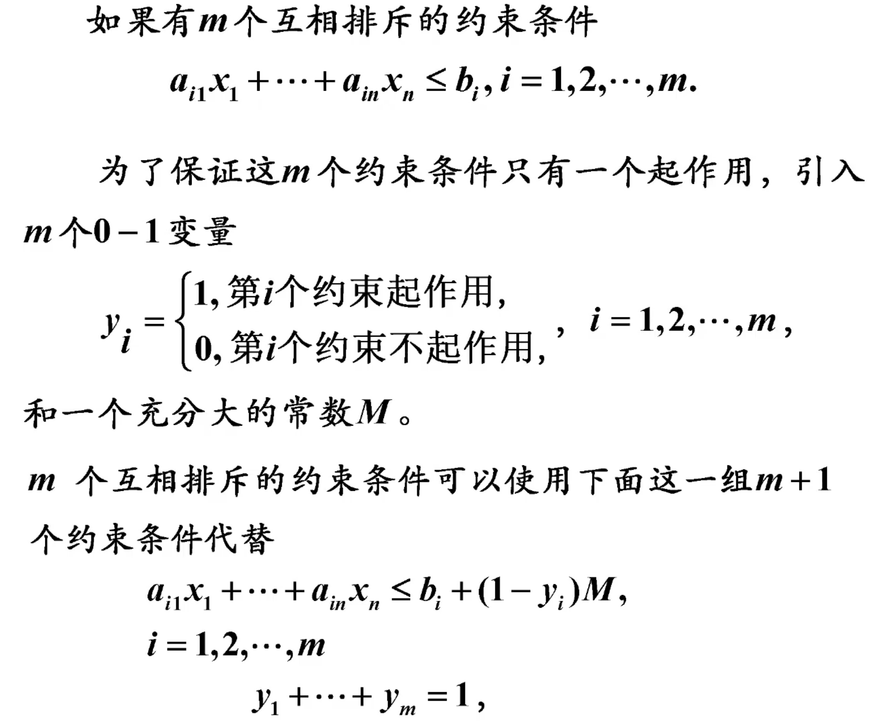
1.相互排斥的约束条件
有两种运输方式可供选择,但只能选择一种运输方式,或者用车运输,或者用船运输。用车运输的约束条件为 5 x 1 + 4 x 2 ≤ 24 5x_1+4x_2≤24 5x1+4x2≤24,用船运输的约束条件为 7 x 1 + 3 x 2 ≤ 45 7x_1+3x_2≤45 7x1+3x2≤45。
即有两个相互排斥的约束条件: 5 x 1 + 4 x 2 ≤ 24 5x_1+4x_2≤24 5x1+4x2≤24 或 7 x 1 + 3 x 2 ≤ 45 7x_1+3x_2≤45 7x1+3x2≤45