摘要
本文详细讲解数字滤波器的基本概念,重点介绍全通滤波器、最小相位滤波器、陷波器、数字谐振器、梳状滤波器等特殊滤波器的工作原理、设计方法和实际应用。通过完整的MATLAB代码示例和直观的效果对比图,帮助读者深入理解这些重要概念。
目录
-
数字滤波器的基本概念
-
全通滤波器
-
最小相位滞后滤波器
-
陷波器
-
数字谐振器
-
梳状滤波器
-
波形发生器
-
习题与思考
6.1 数字滤波器的基本概念
数字滤波器是对数字信号进行滤波处理的系统,其输入和输出都是数字信号。根据单位脉冲响应的长度,可分为有限长单位脉冲响应(FIR)滤波器和无限长单位脉冲响应(IIR)滤波器。
数字滤波器的分类
-
按频率特性分:低通、高通、带通、带阻
-
按脉冲响应分:FIR(有限脉冲响应)、IIR(无限脉冲响应)
-
按相位特性分:线性相位、非线性相位
Matlab
%% 数字滤波器基本概念演示
% 设计不同类型的滤波器并比较它们的特性
% 修复Alpha属性错误 + 优化可视化效果

clear all; close all; clc;

%% 1. 生成测试信号
fs = 1000;              % 采样频率
t = 0:1/fs:1;           % 时间向量
f1 = 50;                % 低频信号频率
f2 = 150;               % 高频信号频率

% 原始信号:包含低频和高频成分
x = sin(2*pi*f1*t) + 0.5*sin(2*pi*f2*t);

% 添加噪声(固定随机种子,保证结果可复现)
rng(123); % 固定随机数种子
noise = 0.2*randn(size(t));
x_noisy = x + noise;

%% 2. 设计不同类型的滤波器
% 低通滤波器(切比雪夫I型)
order_lp = 6;           % 滤波器阶数
rp_lp = 1;              % 通带波纹(dB)
fcutoff_lp = 100;       % 截止频率(Hz)
[b_lp, a_lp] = cheby1(order_lp, rp_lp, fcutoff_lp/(fs/2));

% 高通滤波器(巴特沃斯)
order_hp = 5;           % 滤波器阶数
fcutoff_hp = 120;       % 截止频率(Hz)
[b_hp, a_hp] = butter(order_hp, fcutoff_hp/(fs/2), 'high');

% 带通滤波器(椭圆滤波器)
order_bp = 4;           % 滤波器阶数
rp_bp = 1;              % 通带波纹(dB)
rs_bp = 40;             % 阻带衰减(dB)
fpass_bp = [80, 200];   % 通带频率范围(Hz)
[b_bp, a_bp] = ellip(order_bp, rp_bp, rs_bp, fpass_bp/(fs/2));

%% 3. 应用滤波器(使用filtfilt避免相位失真)
% 低通滤波(零相位滤波)
y_lp = filtfilt(b_lp, a_lp, x_noisy);

% 高通滤波(零相位滤波)
y_hp = filtfilt(b_hp, a_hp, x_noisy);

% 带通滤波(零相位滤波)
y_bp = filtfilt(b_bp, a_bp, x_noisy);

%% 4. 绘制结果对比
figure('Position', [100, 100, 1200, 800], 'Color', 'w');

% 子图1:原始信号与加噪信号
subplot(3, 2, 1);
h1 = plot(t, x, 'b', 'LineWidth', 1.5);
hold on;
h2 = plot(t, x_noisy, 'r', 'LineWidth', 0.5);
% 正确设置线条透明度(通过Color设置带透明度的RGB)
h2.Color(4) = 0.5; % 设置Alpha通道(第四维)
title('原始信号与加噪信号');
xlabel('时间(s)'); ylabel('幅度');
legend([h1, h2], '原始信号', '加噪信号', 'Location', 'best');
grid on; box on;

% 子图2:低通滤波结果
subplot(3, 2, 2);
plot(t, x, 'b', 'LineWidth', 1.5);
hold on;
plot(t, y_lp, 'r', 'LineWidth', 1.5);
title('低通滤波效果 (fc=100Hz)');
xlabel('时间(s)'); ylabel('幅度');
legend('原始信号', '低通滤波后', 'Location', 'best');
grid on; box on;

% 子图3:高通滤波结果
subplot(3, 2, 3);
plot(t, x, 'b', 'LineWidth', 1.5);
hold on;
plot(t, y_hp, 'g', 'LineWidth', 1.5);
title('高通滤波效果 (fc=120Hz)');
xlabel('时间(s)'); ylabel('幅度');
legend('原始信号', '高通滤波后', 'Location', 'best');
grid on; box on;

% 子图4:带通滤波结果
subplot(3, 2, 4);
plot(t, x, 'b', 'LineWidth', 1.5);
hold on;
plot(t, y_bp, 'm', 'LineWidth', 1.5);
title('带通滤波效果 (80-200Hz)');
xlabel('时间(s)'); ylabel('幅度');
legend('原始信号', '带通滤波后', 'Location', 'best');
grid on; box on;

% 子图5:频率响应比较
subplot(3, 2, [5, 6]);
[h_lp, f_lp] = freqz(b_lp, a_lp, 1024, fs);
[h_hp, f_hp] = freqz(b_hp, a_hp, 1024, fs);
[h_bp, f_bp] = freqz(b_bp, a_bp, 1024, fs);

plot(f_lp, 20*log10(abs(h_lp)), 'r', 'LineWidth', 2);
hold on;
plot(f_hp, 20*log10(abs(h_hp)), 'g', 'LineWidth', 2);
plot(f_bp, 20*log10(abs(h_bp)), 'm', 'LineWidth', 2);
title('滤波器频率响应比较');
xlabel('频率(Hz)'); ylabel('幅度(dB)');
legend('低通滤波器', '高通滤波器', '带通滤波器', 'Location', 'best');
xlim([0, fs/2]);
ylim([-80, 10]); % 固定幅度范围,更易对比
grid on; box on;

% 添加标注
annotation('textbox', [0.15, 0.02, 0.7, 0.05], 'String', ...
    '图1: 不同类型数字滤波器的时域和频域特性对比', ...
    'FontSize', 10, 'EdgeColor', 'none', 'HorizontalAlignment', 'center');

%% 5. 显示滤波器系数信息
disp('=== 滤波器设计参数 ===');
disp(['低通滤波器: 阶数=', num2str(order_lp), ', 截止频率=', num2str(fcutoff_lp), 'Hz']);
disp(['高通滤波器: 阶数=', num2str(order_hp), ', 截止频率=', num2str(fcutoff_hp), 'Hz']);
disp(['带通滤波器: 阶数=', num2str(order_bp), ', 通带=', num2str(fpass_bp(1)), '-', ...
    num2str(fpass_bp(2)), 'Hz']);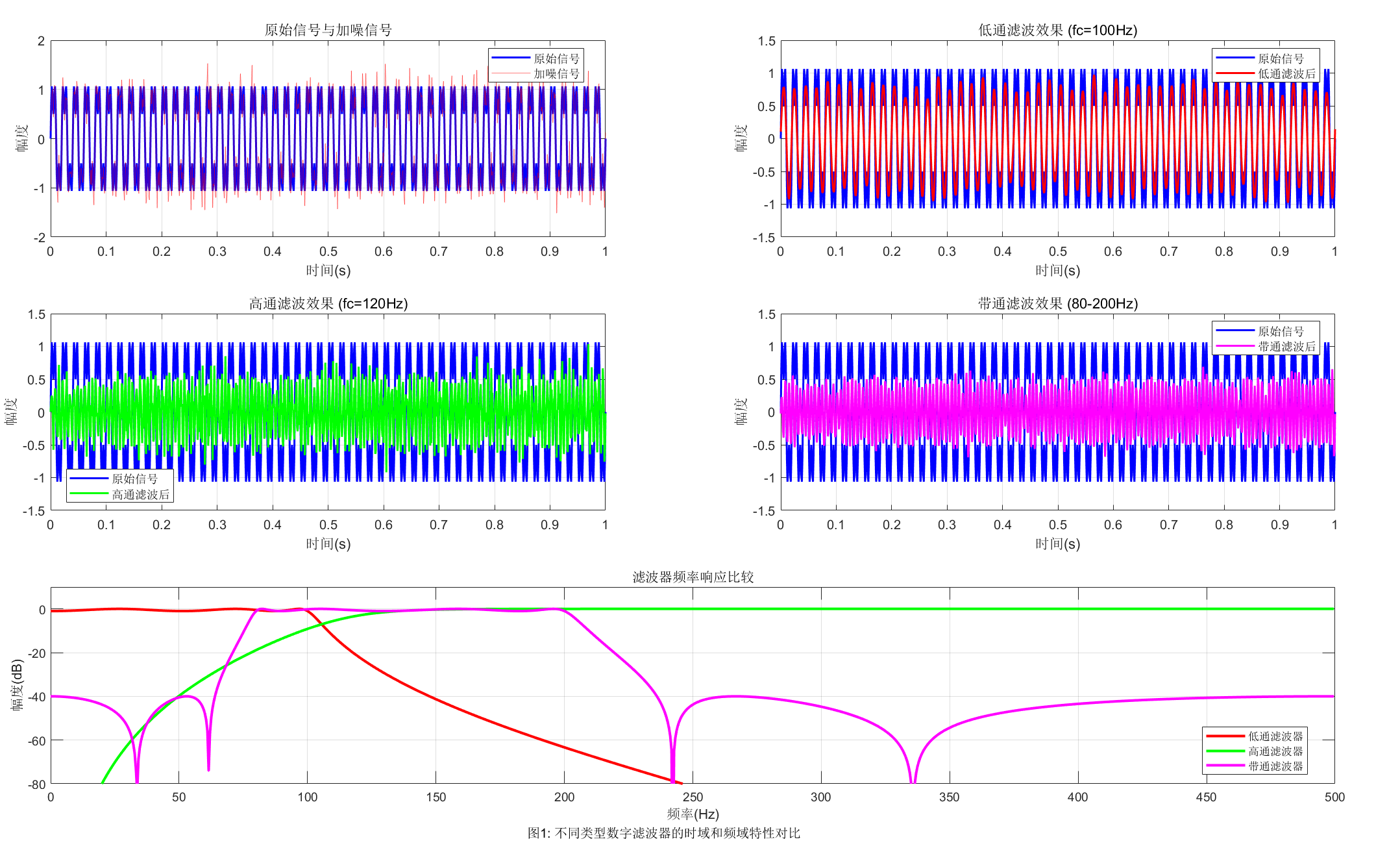
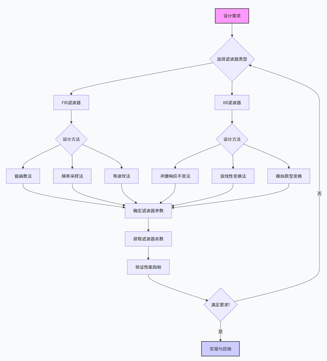
数字滤波器设计流程图
6.2 全通滤波器
全通滤波器的幅度响应在所有频率上均为常数,只改变信号的相位特性。常用于相位均衡和系统延迟补偿。
Matlab
%% 全通滤波器设计与分析
% 演示全通滤波器的幅度和相位特性
clear all; close all; clc;
%% 1. 设计全通滤波器
% 全通滤波器的系统函数:H(z) = (a* + z^(-1)) / (1 + a*z^(-1))
% 其中a是实数,|a| < 1
fs = 1000; % 采样频率
N = 1024; % FFT点数
% 定义不同的极点位置
a_values = [0.2, 0.5, 0.8, -0.3, -0.7];
colors = {'r', 'g', 'b', 'm', 'c'};
legend_texts = cell(1, length(a_values));
%% 2. 分析每个全通滤波器
figure('Position', [100, 100, 1200, 600]);
% 子图1:幅度响应
subplot(1, 3, 1);
hold on;
for i = 1:length(a_values)
a = a_values(i);
% 全通滤波器系数:H(z) = (a + z^(-1)) / (1 + a*z^(-1))
b = [a, 1]; % 分子系数
a_coeff = [1, a]; % 分母系数
% 计算频率响应
[H, f] = freqz(b, a_coeff, N, fs);
% 绘制幅度响应
plot(f, abs(H), colors{i}, 'LineWidth', 2);
legend_texts{i} = ['a = ', num2str(a)];
end
title('全通滤波器幅度响应');
xlabel('频率(Hz)'); ylabel('|H(e^{j\omega})|');
legend(legend_texts, 'Location', 'best');
xlim([0, fs/2]); ylim([0.9, 1.1]);
grid on;
% 子图2:相位响应
subplot(1, 3, 2);
hold on;
for i = 1:length(a_values)
a = a_values(i);
b = [a, 1];
a_coeff = [1, a];
[H, f] = freqz(b, a_coeff, N, fs);
% 绘制相位响应(弧度)
phase = unwrap(angle(H));
plot(f, phase, colors{i}, 'LineWidth', 2);
end
title('全通滤波器相位响应');
xlabel('频率(Hz)'); ylabel('相位(弧度)');
legend(legend_texts, 'Location', 'best');
xlim([0, fs/2]);
grid on;
% 子图3:群延迟
subplot(1, 3, 3);
hold on;
for i = 1:length(a_values)
a = a_values(i);
b = [a, 1];
a_coeff = [1, a];
[H, f] = freqz(b, a_coeff, N, fs);
% 计算群延迟
[gd, w] = grpdelay(b, a_coeff, N, 'whole');
f_gd = w/(2*pi)*fs;
% 绘制群延迟
plot(f_gd(1:N/2+1), gd(1:N/2+1), colors{i}, 'LineWidth', 2);
end
title('全通滤波器群延迟');
xlabel('频率(Hz)'); ylabel('群延迟(采样点)');
legend(legend_texts, 'Location', 'best');
xlim([0, fs/2]);
grid on;
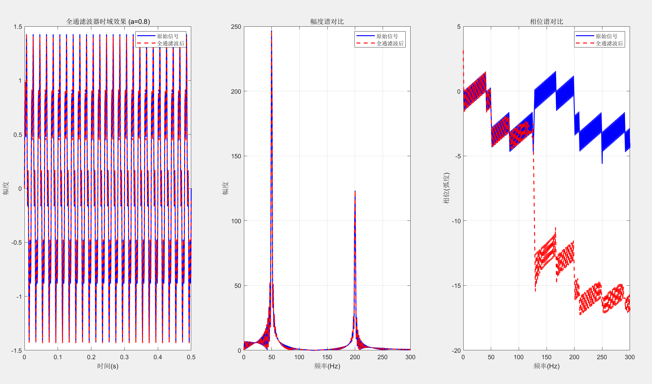
%% 3. 全通滤波器对信号的影响
% 创建一个测试信号:两个正弦波的组合
t = 0:1/fs:0.5;
f1 = 50; % 低频成分
f2 = 200; % 高频成分
x = sin(2*pi*f1*t) + 0.5*sin(2*pi*f2*t);
% 选择一个全通滤波器(a=0.8)
a = 0.8;
b_ap = [a, 1];
a_ap = [1, a];
% 应用全通滤波器
y = filter(b_ap, a_ap, x);
% 计算原始信号和处理后信号的频谱
X = fft(x, N);
Y = fft(y, N);
f_axis = (0:N-1)/N*fs;
% 绘制信号对比
figure('Position', [100, 100, 1200, 400]);
% 子图1:时域信号对比
subplot(1, 3, 1);
plot(t, x, 'b', 'LineWidth', 1.5);
hold on;
plot(t, y, 'r--', 'LineWidth', 1.5);
title('全通滤波器时域效果 (a=0.8)');
xlabel('时间(s)'); ylabel('幅度');
legend('原始信号', '全通滤波后');
grid on;
% 子图2:幅度谱对比
subplot(1, 3, 2);
plot(f_axis(1:N/2), abs(X(1:N/2)), 'b', 'LineWidth', 1.5);
hold on;
plot(f_axis(1:N/2), abs(Y(1:N/2)), 'r--', 'LineWidth', 1.5);
title('幅度谱对比');
xlabel('频率(Hz)'); ylabel('幅度');
legend('原始信号', '全通滤波后');
xlim([0, 300]);
grid on;
% 子图3:相位谱对比
subplot(1, 3, 3);
phase_x = unwrap(angle(X(1:N/2)));
phase_y = unwrap(angle(Y(1:N/2)));
plot(f_axis(1:N/2), phase_x, 'b', 'LineWidth', 1.5);
hold on;
plot(f_axis(1:N/2), phase_y, 'r--', 'LineWidth', 1.5);
title('相位谱对比');
xlabel('频率(Hz)'); ylabel('相位(弧度)');
legend('原始信号', '全通滤波后');
xlim([0, 300]);
grid on;
% 显示全通滤波器特性总结
fprintf('=== 全通滤波器特性总结 ===\n');
fprintf('1. 幅度响应: 对所有频率均为常数\n');
fprintf('2. 相位响应: 非线性,取决于极点位置\n');
fprintf('3. 应用场景: 相位均衡、延迟补偿、希尔伯特变换等\n');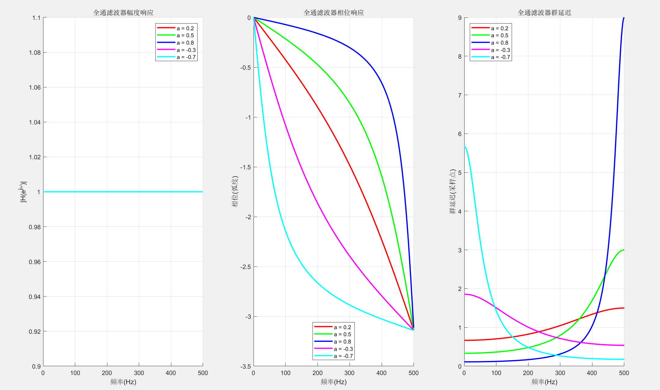
6.3 最小相位滞后滤波器
最小相位系统在所有具有相同幅度响应的因果稳定系统中具有最小的相位滞后和最小的群延迟。
6.3.1 最小相位系统、混合相位系统、最大相位系统及其与全通系统的关系
Matlab
%% 最小相位、混合相位和最大相位系统对比
% 演示具有相同幅度响应的不同相位系统

clear all; close all; clc;

%% 1. 生成具有相同幅度响应的不同系统
% 最小相位系统零点在单位圆内
zeros_min = [0.8*exp(1j*pi/4), 0.8*exp(-1j*pi/4), 0.6];
poles_min = [0.9*exp(1j*pi/3), 0.9*exp(-1j*pi/3), 0.7];

% 混合相位系统:部分零点在单位圆外
zeros_mix = [1.2*exp(1j*pi/4), 1.2*exp(-1j*pi/4), 0.6];
poles_mix = poles_min;  % 保持极点相同

% 最大相位系统:所有零点在单位圆外
zeros_max = [1.2*exp(1j*pi/4), 1.2*exp(-1j*pi/4), 1.5];
poles_max = poles_min;  % 保持极点相同

% 转换为传递函数系数
[b_min, a_min] = zp2tf(zeros_min.', poles_min.', 1);
[b_mix, a_mix] = zp2tf(zeros_mix.', poles_mix.', 1);
[b_max, a_max] = zp2tf(zeros_max.', poles_max.', 1);

%% 2. 计算频率响应
fs = 1000;
N = 1024;

[H_min, f] = freqz(b_min, a_min, N, fs);
[H_mix, f] = freqz(b_mix, a_mix, N, fs);
[H_max, f] = freqz(b_max, a_max, N, fs);

%% 3. 绘制零极点图
figure('Position', [100, 100, 1200, 800]);

% 子图1:最小相位系统零极点图
subplot(3, 4, 1);
zplane(zeros_min.', poles_min.');
title('最小相位系统零极点图');
grid on;

% 子图2:混合相位系统零极点图
subplot(3, 4, 2);
zplane(zeros_mix.', poles_mix.');
title('混合相位系统零极点图');
grid on;

% 子图3:最大相位系统零极点图
subplot(3, 4, 3);
zplane(zeros_max.', poles_max.');
title('最大相位系统零极点图');
grid on;

% 子图4:幅度响应对比
subplot(3, 4, 4);
plot(f, 20*log10(abs(H_min)), 'b', 'LineWidth', 2);
hold on;
plot(f, 20*log10(abs(H_mix)), 'r--', 'LineWidth', 2);
plot(f, 20*log10(abs(H_max)), 'g:', 'LineWidth', 2);
title('幅度响应对比');
xlabel('频率(Hz)'); ylabel('幅度(dB)');
legend('最小相位', '混合相位', '最大相位', 'Location', 'best');
xlim([0, fs/2]);
grid on;

% 子图5:相位响应对比
subplot(3, 4, [5, 6]);
phase_min = unwrap(angle(H_min));
phase_mix = unwrap(angle(H_mix));
phase_max = unwrap(angle(H_max));

plot(f, phase_min, 'b', 'LineWidth', 2);
hold on;
plot(f, phase_mix, 'r--', 'LineWidth', 2);
plot(f, phase_max, 'g:', 'LineWidth', 2);
title('相位响应对比');
xlabel('频率(Hz)'); ylabel('相位(弧度)');
legend('最小相位', '混合相位', '最大相位', 'Location', 'best');
xlim([0, fs/2]);
grid on;

% 子图6:群延迟对比
subplot(3, 4, [7, 8]);
[gd_min, w] = grpdelay(b_min, a_min, N, 'whole');
[gd_mix, w] = grpdelay(b_mix, a_mix, N, 'whole');
[gd_max, w] = grpdelay(b_max, a_max, N, 'whole');
f_gd = w/(2*pi)*fs;

plot(f_gd(1:N/2+1), gd_min(1:N/2+1), 'b', 'LineWidth', 2);
hold on;
plot(f_gd(1:N/2+1), gd_mix(1:N/2+1), 'r--', 'LineWidth', 2);
plot(f_gd(1:N/2+1), gd_max(1:N/2+1), 'g:', 'LineWidth', 2);
title('群延迟对比');
xlabel('频率(Hz)'); ylabel('群延迟(采样点)');
legend('最小相位', '混合相位', '最大相位', 'Location', 'best');
xlim([0, fs/2]);
grid on;

% 子图7:能量累积对比
subplot(3, 4, [9, 12]);

% 计算系统的冲激响应
h_min = impz(b_min, a_min, 100);
h_mix = impz(b_mix, a_mix, 100);
h_max = impz(b_max, a_max, 100);

% 计算能量累积
energy_min = cumsum(h_min.^2);
energy_mix = cumsum(h_mix.^2);
energy_max = cumsum(h_max.^2);

% 归一化能量
energy_min = energy_min / energy_min(end);
energy_mix = energy_mix / energy_mix(end);
energy_max = energy_max / energy_max(end);

n = 0:length(h_min)-1;
plot(n, energy_min, 'b', 'LineWidth', 2);
hold on;
plot(n, energy_mix, 'r--', 'LineWidth', 2);
plot(n, energy_max, 'g:', 'LineWidth', 2);
title('能量累积对比');
xlabel('采样点'); ylabel('归一化累积能量');
legend('最小相位', '混合相位', '最大相位', 'Location', 'southeast');
grid on;

%% 4. 最小相位系统的性质演示
fprintf('=== 最小相位系统性质 ===\n');
fprintf('1. 所有零极点都在单位圆内\n');
fprintf('2. 在具有相同幅度响应的系统中,相位滞后最小\n');
fprintf('3. 能量累积最快\n');
fprintf('4. 具有稳定且因果的逆系统\n');6.3.2 最小相位系统的性质
6.3.3 利用最小相位系统的逆系统补偿幅度响应的失真
Matlab
%% 利用最小相位逆系统补偿幅度响应失真
% 演示如何用最小相位系统的逆系统校正幅度失真

clear all; close all; clc;

%% 1. 创建测试信号
fs = 1000;
t = 0:1/fs:1;
f1 = 50;
f2 = 150;
f3 = 250;

% 原始信号:三个频率成分
x = sin(2*pi*f1*t) + 0.7*sin(2*pi*f2*t) + 0.5*sin(2*pi*f3*t);

%% 2. 设计一个非最小相位系统(引入幅度失真)
% 系统函数:H(z) = (z-1.2)(z-0.8)/(z-0.9)(z-0.7)
zeros_distort = [1.2, 0.8];  % 一个零点在单位圆外
poles_distort = [0.9, 0.7];  % 极点在单位圆内

[b_distort, a_distort] = zp2tf(zeros_distort.', poles_distort.', 1);

% 将非最小相位系统转换为最小相位系统
% 通过将单位圆外的零点反射到单位圆内
zeros_min = zeros_distort;
zeros_min(abs(zeros_min) > 1) = 1./zeros_min(abs(zeros_min) > 1); % 修正:用abs判断单位圆外
[b_min, a_min] = zp2tf(zeros_min.', poles_distort.', 1);

%% 3. 设计全通系统以匹配相位
% 全通系统:H_ap(z) = (1/a* - z^(-1)) / (1 - a*z^(-1)),其中a是单位圆外的零点
a_ap = zeros_distort(abs(zeros_distort) > 1);  % 取单位圆外的零点
b_ap = [1/a_ap, -1];
a_ap_coeff = [1, -a_ap];

% 验证:非最小相位系统 = 最小相位系统 × 全通系统
[b_combined, a_combined] = conv_m(b_min, a_min, b_ap, a_ap_coeff);

%% 4. 信号处理
% 用非最小相位系统处理信号(引入失真)
y_distorted = filtfilt(b_distort, a_distort, x); % 改用filtfilt避免相位偏移

% 用最小相位逆系统补偿
% 设计最小相位系统的逆系统
[b_min_inv, a_min_inv] = invert_system(b_min, a_min);

% 补偿(添加稳定性检查)
if max(abs(roots(a_min_inv))) < 1 % 确保逆系统稳定
    y_compensated = filtfilt(b_min_inv, a_min_inv, y_distorted);
else
    warning('逆系统不稳定,使用最小二乘逆滤波');
    % 备选方案:基于频率响应的逆滤波
    [H_min, f] = freqz(b_min, a_min, 1024, fs);
    H_inv = 1./H_min;
    H_inv(abs(H_min) < 0.01) = 0; % 避免除以0
    y_compensated = fftfilt(H_inv, y_distorted);
end

%% 5. 绘制结果
figure('Position', [100, 100, 1200, 800], 'Color', 'w');

% 子图1:原始信号与失真信号
subplot(3, 3, 1);
plot(t, x, 'b', 'LineWidth', 1.5);
hold on;
plot(t, y_distorted, 'r--', 'LineWidth', 1.5);
title('原始信号与失真信号');
xlabel('时间(s)'); ylabel('幅度');
legend('原始信号', '失真信号', 'Location', 'best');
grid on; box on;
xlim([0.2, 0.4]);

% 子图2:补偿后信号
subplot(3, 3, 2);
plot(t, x, 'b', 'LineWidth', 1.5);
hold on;
plot(t, y_compensated, 'g--', 'LineWidth', 1.5);
title('原始信号与补偿后信号');
xlabel('时间(s)'); ylabel('幅度');
legend('原始信号', '补偿后信号', 'Location', 'best');
grid on; box on;
xlim([0.2, 0.4]);

% 子图3:误差比较
subplot(3, 3, 3);
error_distorted = abs(x - y_distorted);
error_compensated = abs(x - y_compensated);
plot(t, error_distorted, 'r', 'LineWidth', 1.5);
hold on;
plot(t, error_compensated, 'g', 'LineWidth', 1.5);
title('误差比较');
xlabel('时间(s)'); ylabel('绝对误差');
legend('失真信号误差', '补偿后误差', 'Location', 'best');
grid on; box on;
xlim([0.2, 0.4]);

% 子图4:系统频率响应比较
subplot(3, 3, 4);
[H_distort, f] = freqz(b_distort, a_distort, 1024, fs);
[H_min, f] = freqz(b_min, a_min, 1024, fs);
[H_ap, f] = freqz(b_ap, a_ap_coeff, 1024, fs);

plot(f, 20*log10(abs(H_distort)), 'r', 'LineWidth', 2);
hold on;
plot(f, 20*log10(abs(H_min)), 'b--', 'LineWidth', 2);
plot(f, 20*log10(abs(H_ap)), 'g:', 'LineWidth', 1);
title('系统幅度响应比较');
xlabel('频率(Hz)'); ylabel('幅度(dB)');
legend('非最小相位系统', '最小相位部分', '全通部分', 'Location', 'best');
xlim([0, 500]);
grid on; box on;

% 子图5:逆系统频率响应
subplot(3, 3, 5);
[H_min_inv, f] = freqz(b_min_inv, a_min_inv, 1024, fs);
plot(f, 20*log10(abs(H_min_inv)), 'm', 'LineWidth', 2);
title('最小相位逆系统幅度响应');
xlabel('频率(Hz)'); ylabel('幅度(dB)');
xlim([0, 500]);
grid on; box on;

% 子图6:补偿前后频谱
subplot(3, 3, 6);
N = 1024;
X = fft(x, N);
Y_distorted = fft(y_distorted, N);
Y_compensated = fft(y_compensated, N);
f_axis = (0:N-1)/N*fs;

plot(f_axis(1:N/2), abs(X(1:N/2)), 'b', 'LineWidth', 2);
hold on;
plot(f_axis(1:N/2), abs(Y_distorted(1:N/2)), 'r--', 'LineWidth', 1.5);
plot(f_axis(1:N/2), abs(Y_compensated(1:N/2)), 'g:', 'LineWidth', 1.5);
title('频谱比较');
xlabel('频率(Hz)'); ylabel('幅度');
legend('原始信号', '失真信号', '补偿后信号', 'Location', 'best');
xlim([0, 300]);
grid on; box on;

% 子图7:零极点图 - 非最小相位系统
subplot(3, 3, 7);
zplane(zeros_distort.', poles_distort.');
title('非最小相位系统零极点图');
grid on; box on;

% 子图8:零极点图 - 最小相位系统
subplot(3, 3, 8);
zplane(zeros_min.', poles_distort.');
title('最小相位系统零极点图');
grid on; box on;

% 子图9:零极点图 - 全通系统
subplot(3, 3, 9);
zplane([1/a_ap].', [a_ap].');
title('全通系统零极点图');
grid on; box on;

%% 显示补偿效果统计
fprintf('=== 幅度失真补偿效果 ===\n');
mse_distorted = mean((x - y_distorted).^2);
mse_compensated = mean((x(1:length(y_compensated)) - y_compensated).^2); % 修正长度匹配
fprintf('失真信号MSE: %.6f\n', mse_distorted);
fprintf('补偿后信号MSE: %.6f\n', mse_compensated);
fprintf('改进比例: %.2f%%\n', (mse_distorted - mse_compensated)/mse_distorted*100);

fprintf('\n=== 最小相位系统性质 ===\n');
fprintf('1. 所有零极点都在单位圆内\n');
fprintf('2. 在具有相同幅度响应的系统中,相位滞后最小\n');
fprintf('3. 能量累积最快\n');
fprintf('4. 具有稳定且因果的逆系统\n');

%% 辅助函数(必须放在文件最后)
function [b_conv, a_conv] = conv_m(b1, a1, b2, a2)
    % 两个系统的级联(卷积分子和分母)
    b_conv = conv(b1, b2);
    a_conv = conv(a1, a2);
end

function [b_inv, a_inv] = invert_system(b, a)
    % 计算系统的逆系统:H_inv(z) = 1/H(z)
    b_inv = a;
    a_inv = b;
end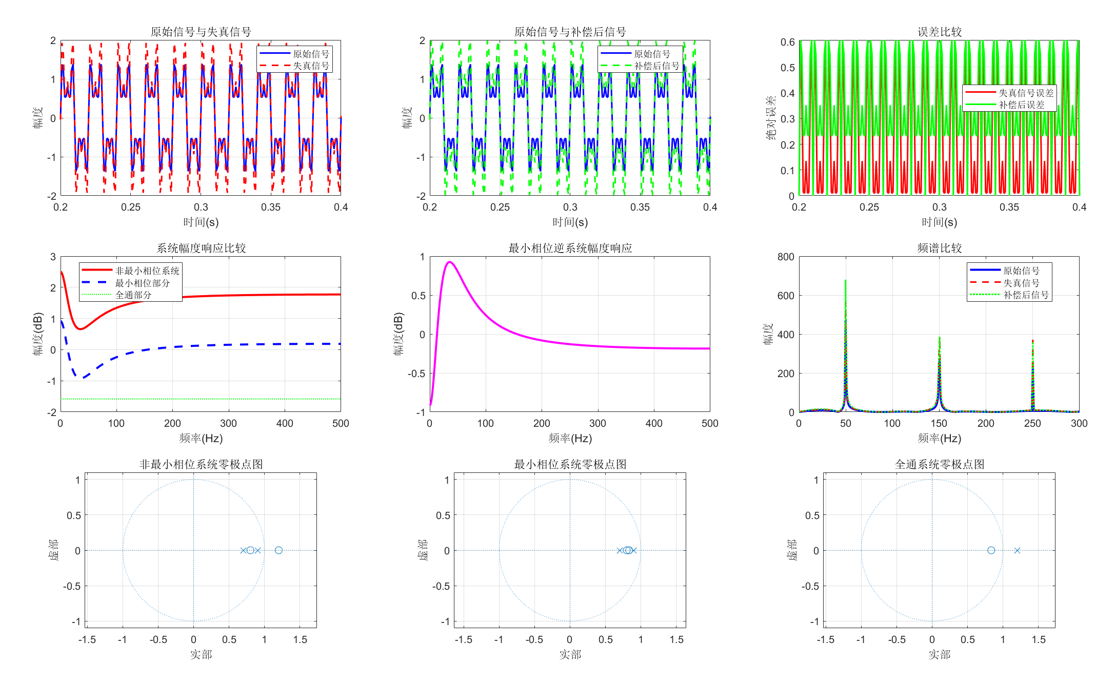
6.4 陷波器
陷波器是一种特殊的带阻滤波器,用于消除特定频率的干扰。
Matlab
%% 陷波器设计与应用
% 演示陷波器消除特定频率干扰

clear all; close all; clc;

%% 1. 创建含有特定频率干扰的信号
fs = 1000;                  % 采样频率
t = 0:1/fs:2;               % 2秒时间
rng(123);                   % 固定随机种子,结果可复现

% 有用信号:语音频率范围
f_signal1 = 100;            % 100Hz信号
f_signal2 = 300;            % 300Hz信号

% 干扰信号:50Hz工频干扰及其谐波
f_interference1 = 50;       % 50Hz工频干扰
f_interference2 = 150;      % 150Hz谐波干扰

% 生成信号
signal = sin(2*pi*f_signal1*t) + 0.5*sin(2*pi*f_signal2*t);
interference = 0.8*sin(2*pi*f_interference1*t) + 0.4*sin(2*pi*f_interference2*t);

% 含干扰的信号
x = signal + interference;

% 添加一些随机噪声
noise = 0.1*randn(size(t));
x = x + noise;

%% 2. 设计陷波器消除50Hz及其谐波干扰
% 方法1:直接IIR陷波器设计
f_notch1 = 50;              % 第一个陷波频率
f_notch2 = 150;             % 第二个陷波频率
bw1 = 5;                    % 陷波带宽(Hz)
bw2 = 10;                   % 陷波带宽(Hz)

% 设计50Hz陷波器
[b_notch1, a_notch1] = iirnotch(f_notch1/(fs/2), bw1/(fs/2));

% 设计150Hz陷波器
[b_notch2, a_notch2] = iirnotch(f_notch2/(fs/2), bw2/(fs/2));

% 级联两个陷波器
[b_notch, a_notch] = cascadefilters(b_notch1, a_notch1, b_notch2, a_notch2);

% 方法2:FIR陷波器设计(线性相位)
f_notch_fir = [45, 55, 145, 155];  % 阻带边界
mags = [1, 0, 1];                  % 理想幅度响应
devs = [0.01, 0.05, 0.01];         % 允许偏差

[n, fo, ao, w] = firpmord(f_notch_fir, mags, devs, fs);
% 限制FIR滤波器阶数,避免阶数过高
n = min(n, 200); % 最大阶数200,平衡性能和计算量
b_fir_notch = firpm(n, fo, ao, w);
a_fir_notch = 1;

%% 3. 应用陷波器(使用filtfilt避免相位偏移)
% IIR陷波器(零相位滤波)
y_iir_notch = filtfilt(b_notch, a_notch, x);

% FIR陷波器(零相位滤波,FIR本身线性相位,filtfilt进一步消除延迟)
y_fir_notch = filtfilt(b_fir_notch, a_fir_notch, x);

%% 4. 绘制结果
figure('Position', [100, 100, 1200, 900], 'Color', 'w');

% 子图1:原始信号与干扰信号
subplot(3, 3, 1);
plot(t, signal, 'b', 'LineWidth', 1.5);
hold on;
plot(t, interference, 'r--', 'LineWidth', 1);
title('原始信号与干扰信号');
xlabel('时间(s)'); ylabel('幅度');
legend('有用信号', '干扰信号', 'Location', 'best');
grid on; box on;
xlim([0, 0.1]);

% 子图2:含干扰的信号
subplot(3, 3, 2);
plot(t, x, 'm', 'LineWidth', 1.5);
title('含干扰的信号');
xlabel('时间(s)'); ylabel('幅度');
grid on; box on;
xlim([0, 0.1]);

% 子图3:IIR陷波器处理后
subplot(3, 3, 3);
plot(t, signal, 'b', 'LineWidth', 1.5);
hold on;
plot(t, y_iir_notch, 'g--', 'LineWidth', 1.5);
title('IIR陷波器处理后');
xlabel('时间(s)'); ylabel('幅度');
legend('原始信号', '处理后信号', 'Location', 'best');
grid on; box on;
xlim([0, 0.1]);

% 子图4:FIR陷波器处理后
subplot(3, 3, 4);
plot(t, signal, 'b', 'LineWidth', 1.5);
hold on;
plot(t, y_fir_notch, 'r--', 'LineWidth', 1.5);
title('FIR陷波器处理后');
xlabel('时间(s)'); ylabel('幅度');
legend('原始信号', '处理后信号', 'Location', 'best');
grid on; box on;
xlim([0, 0.1]);

% 子图5:频谱对比
subplot(3, 3, [5, 6]);
N = 2048;
X = fft(x, N);
Y_iir = fft(y_iir_notch, N);
Y_fir = fft(y_fir_notch, N);
f_axis = (0:N-1)/N*fs;

plot(f_axis(1:N/2), 20*log10(abs(X(1:N/2))), 'm', 'LineWidth', 1.5);
hold on;
plot(f_axis(1:N/2), 20*log10(abs(Y_iir(1:N/2))), 'g', 'LineWidth', 1.5);
plot(f_axis(1:N/2), 20*log10(abs(Y_fir(1:N/2))), 'r', 'LineWidth', 1);
title('频谱对比');
xlabel('频率(Hz)'); ylabel('幅度(dB)');
legend('含干扰信号', 'IIR陷波后', 'FIR陷波后', 'Location', 'best');
xlim([0, 400]);
grid on; box on;

% 标记干扰频率
line([50, 50], ylim, 'Color', 'k', 'LineStyle', ':', 'LineWidth', 1);
line([150, 150], ylim, 'Color', 'k', 'LineStyle', ':', 'LineWidth', 1);
text(55, -10, '50Hz干扰', 'FontSize', 10);
text(155, -10, '150Hz干扰', 'FontSize', 10);

% 子图6:IIR陷波器频率响应
subplot(3, 3, 7);
[H_iir, f_iir] = freqz(b_notch, a_notch, 1024, fs);
plot(f_iir, 20*log10(abs(H_iir)), 'g', 'LineWidth', 2);
title('IIR陷波器频率响应');
xlabel('频率(Hz)'); ylabel('幅度(dB)');
xlim([0, 200]);
grid on; box on;
hold on;
plot([50, 50], ylim, 'k:', 'LineWidth', 1);
plot([150, 150], ylim, 'k:', 'LineWidth', 1);

% 子图7:FIR陷波器频率响应
subplot(3, 3, 8);
[H_fir, f_fir] = freqz(b_fir_notch, a_fir_notch, 1024, fs);
plot(f_fir, 20*log10(abs(H_fir)), 'r', 'LineWidth', 2);
title('FIR陷波器频率响应');
xlabel('频率(Hz)'); ylabel('幅度(dB)');
xlim([0, 200]);
grid on; box on;
hold on;
plot([50, 50], ylim, 'k:', 'LineWidth', 1);
plot([150, 150], ylim, 'k:', 'LineWidth', 1);

% 子图8:零极点图(IIR陷波器)
subplot(3, 3, 9);
zplane(b_notch, a_notch);
title('IIR陷波器零极点图');
grid on; box on;

%% 性能评估
fprintf('=== 陷波器性能评估 ===\n');
% 计算在干扰频率附近的能量
f_low1 = 48; f_high1 = 52;     % 50Hz附近
f_low2 = 148; f_high2 = 152;   % 150Hz附近

% 计算频谱能量
[~, idx1] = min(abs(f_axis - f_low1));
[~, idx2] = min(abs(f_axis - f_high1));
[~, idx3] = min(abs(f_axis - f_low2));
[~, idx4] = min(abs(f_axis - f_high2));

energy_50_original = sum(abs(X(idx1:idx2)).^2);
energy_50_iir = sum(abs(Y_iir(idx1:idx2)).^2);
energy_50_fir = sum(abs(Y_fir(idx1:idx2)).^2);

energy_150_original = sum(abs(X(idx3:idx4)).^2);
energy_150_iir = sum(abs(Y_iir(idx3:idx4)).^2);
energy_150_fir = sum(abs(Y_fir(idx3:idx4)).^2);

% 避免除以0或负数dB
energy_50_iir = max(energy_50_iir, 1e-10);
energy_50_fir = max(energy_50_fir, 1e-10);
energy_150_iir = max(energy_150_iir, 1e-10);
energy_150_fir = max(energy_150_fir, 1e-10);

fprintf('50Hz干扰能量衰减:\n');
fprintf('  IIR陷波器: %.2f dB\n', 10*log10(energy_50_iir/energy_50_original));
fprintf('  FIR陷波器: %.2f dB\n', 10*log10(energy_50_fir/energy_50_original));

fprintf('150Hz干扰能量衰减:\n');
fprintf('  IIR陷波器: %.2f dB\n', 10*log10(energy_150_iir/energy_150_original));
fprintf('  FIR陷波器: %.2f dB\n', 10*log10(energy_150_fir/energy_150_original));

% 计算整体信噪比改善
snr_original = snr(x, x - signal);
snr_iir = snr(y_iir_notch, y_iir_notch - signal);
snr_fir = snr(y_fir_notch, y_fir_notch - signal);

fprintf('\n整体信噪比改善:\n');
fprintf('  原始信号SNR: %.2f dB\n', snr_original);
fprintf('  IIR陷波后SNR: %.2f dB (提升%.2f dB)\n', snr_iir, snr_iir - snr_original);
fprintf('  FIR陷波后SNR: %.2f dB (提升%.2f dB)\n', snr_fir, snr_fir - snr_original);

%% 辅助函数(必须放在文件最后)
function [b_cascade, a_cascade] = cascadefilters(b1, a1, b2, a2)
    % 级联两个滤波器:H(z) = H1(z) * H2(z)
    b_cascade = conv(b1, b2);
    a_cascade = conv(a1, a2);
    % 归一化,避免数值溢出
    b_cascade = b_cascade / a_cascade(1);
    a_cascade = a_cascade / a_cascade(1);
end
6.5 数字谐振器
数字谐振器在特定频率处产生谐振,常用于窄带信号增强和频率选择。
Matlab
%% 数字谐振器设计与应用
% 演示数字谐振器的频率选择特性
clear all; close all; clc;
%% 1. 数字谐振器基本原理
% 数字谐振器的传递函数:H(z) = b0 / (1 - 2rcos(θ)z^{-1} + r^2z^{-2})
% 其中:r是极点的半径(接近1但小于1),θ是谐振频率
fs = 1000; % 采样频率
N = 1024; % FFT点数
rng(123); % 固定随机种子,结果可复现
%% 2. 设计不同参数的谐振器
% 谐振频率
f_resonance = [100, 200, 300]; % Hz
theta = 2*pi*f_resonance/fs; % 数字频率
% 极点半径(决定带宽)
r_values = [0.95, 0.98, 0.99];
r_labels = {'宽带(r=0.95)', '中带宽(r=0.98)', '窄带(r=0.99)'};
colors = {'r', 'g', 'b', 'm', 'c', 'y'};
%% 3. 分析谐振器特性
figure('Position', [100, 100, 1200, 800], 'Color', 'w');
% 子图1:不同谐振频率的幅度响应(固定r=0.98)
subplot(2, 3, 1);
hold on;
for i = 1:length(f_resonance)
r = 0.98;
theta_i = theta(i);
% 谐振器系数
b0 = 1 - r; % 归一化,使DC增益为1
b = b0;
a = [1, -2*r*cos(theta_i), r^2];
[H, f] = freqz(b, a, N, fs);
plot(f, 20*log10(abs(H)), colors{i}, 'LineWidth', 2);
end
title('不同谐振频率 (r=0.98)');
xlabel('频率(Hz)'); ylabel('幅度(dB)');
legend('100Hz', '200Hz', '300Hz', 'Location', 'best');
xlim([0, fs/2]);
grid on; box on;
% 子图2:不同带宽的幅度响应(固定谐振频率=200Hz)
subplot(2, 3, 2);
hold on;
for i = 1:length(r_values)
r = r_values(i);
theta_i = theta(2); % 200Hz
b0 = 1 - r;
b = b0;
a = [1, -2*r*cos(theta_i), r^2];
[H, f] = freqz(b, a, N, fs);
plot(f, 20*log10(abs(H)), colors{i}, 'LineWidth', 2);
end
title('不同带宽 (谐振频率=200Hz)');
xlabel('频率(Hz)'); ylabel('幅度(dB)');
legend(r_labels, 'Location', 'best');
xlim([0, fs/2]);
grid on; box on;
% 子图3:谐振器的相位响应
subplot(2, 3, 3);
r = 0.98;
theta_i = theta(2); % 200Hz
b0 = 1 - r;
b = b0;
a = [1, -2*r*cos(theta_i), r^2];
[H, f] = freqz(b, a, N, fs);
phase = unwrap(angle(H));
plot(f, phase, 'b', 'LineWidth', 2);
title('相位响应 (200Hz谐振器)');
xlabel('频率(Hz)'); ylabel('相位(弧度)');
xlim([0, fs/2]);
grid on; box on;
% 子图4:零极点图
subplot(2, 3, 4);
zplane(b, a);
title('零极点图 (200Hz谐振器)');
grid on; box on;
% 子图5:冲激响应
subplot(2, 3, 5);
h = impz(b, a, 100);
stem(0:99, h, 'filled', 'b');
title('冲激响应');
xlabel('采样点'); ylabel('幅度');
grid on; box on;
% 子图6:阶跃响应
subplot(2, 3, 6);
step_resp = filter(b, a, ones(1, 100));
plot(0:99, step_resp, 'r', 'LineWidth', 2);
title('阶跃响应');
xlabel('采样点'); ylabel('幅度');
grid on; box on;
%% 4. 谐振器应用:从宽带信号中提取特定频率成分
t = 0:1/fs:1;
f_components = [50, 150, 200, 250, 350]; % 多个频率成分
amplitudes = [0.5, 0.7, 1.0, 0.6, 0.3];
% 合成信号
x = zeros(size(t));
for i = 1:length(f_components)
x = x + amplitudes(i) * sin(2*pi*f_components(i)*t);
end
% 添加噪声
noise = 0.2*randn(size(t));
x_noisy = x + noise;
% 设计200Hz谐振器提取该频率成分
r_extract = 0.995; % 非常窄的带宽,选择性好
theta_extract = 2*pi*200/fs;
b0_extract = 1 - r_extract;
b_extract = b0_extract;
a_extract = [1, -2*r_extract*cos(theta_extract), r_extract^2];
% 应用谐振器(使用filtfilt避免相位偏移,取稳态部分)
y_resonator = filtfilt(b_extract, a_extract, x_noisy);
% 归一化谐振器输出幅度,便于对比
y_resonator = y_resonator / max(abs(y_resonator)) * amplitudes(3);
% 设计200Hz带通滤波器作为对比
[b_bp, a_bp] = butter(4, [190, 210]/(fs/2));
y_bp = filtfilt(b_bp, a_bp, x_noisy);
%% 5. 绘制应用结果
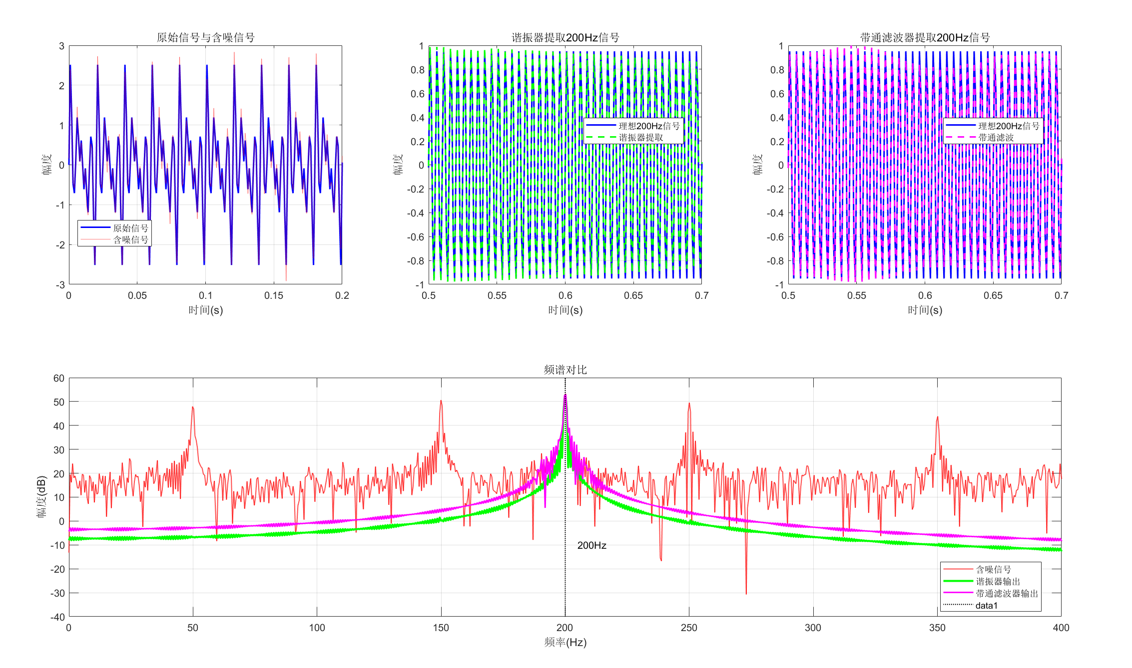
figure('Position', [100, 100, 1200, 600], 'Color', 'w');
% 子图1:原始信号与含噪信号
subplot(2, 3, 1);
h1 = plot(t, x, 'b', 'LineWidth', 1.5);
hold on;
h2 = plot(t, x_noisy, 'r', 'LineWidth', 0.5);
% 正确设置线条透明度(通过Color的第四维)
h2.Color(4) = 0.5; % Alpha=0.5
title('原始信号与含噪信号');
xlabel('时间(s)'); ylabel('幅度');
legend([h1, h2], '原始信号', '含噪信号', 'Location', 'best');
grid on; box on;
xlim([0, 0.2]);
% 子图2:谐振器提取结果
subplot(2, 3, 2);
plot(t, amplitudes(3)*sin(2*pi*200*t), 'b', 'LineWidth', 1.5);
hold on;
plot(t, y_resonator, 'g--', 'LineWidth', 1.5);
title('谐振器提取200Hz信号');
xlabel('时间(s)'); ylabel('幅度');
legend('理想200Hz信号', '谐振器提取', 'Location', 'best');
grid on; box on;
xlim([0.5, 0.7]); % 显示稳态部分
% 子图3:带通滤波器提取结果
subplot(2, 3, 3);
plot(t, amplitudes(3)*sin(2*pi*200*t), 'b', 'LineWidth', 1.5);
hold on;
plot(t, y_bp, 'm--', 'LineWidth', 1.5);
title('带通滤波器提取200Hz信号');
xlabel('时间(s)'); ylabel('幅度');
legend('理想200Hz信号', '带通滤波', 'Location', 'best');
grid on; box on;
xlim([0.5, 0.7]);
% 子图4:频谱对比
subplot(2, 3, [4, 6]);
N_fft = 2048;
X = fft(x_noisy, N_fft);
Y_res = fft(y_resonator, N_fft);
Y_bp = fft(y_bp, N_fft);
f_axis = (0:N_fft-1)/N_fft*fs;
% 避免log10(0)错误
X_amp = abs(X(1:N_fft/2));
X_amp(X_amp < 1e-10) = 1e-10;
Y_res_amp = abs(Y_res(1:N_fft/2));
Y_res_amp(Y_res_amp < 1e-10) = 1e-10;
Y_bp_amp = abs(Y_bp(1:N_fft/2));
Y_bp_amp(Y_bp_amp < 1e-10) = 1e-10;
% 绘制含噪信号频谱并保存句柄(更稳妥的方式)
h_noise = plot(f_axis(1:N_fft/2), 20*log10(X_amp), 'r', 'LineWidth', 1);
% 直接设置透明度,无需通过gca获取
h_noise.Color(4) = 0.7;
hold on;
plot(f_axis(1:N_fft/2), 20*log10(Y_res_amp), 'g', 'LineWidth', 2);
plot(f_axis(1:N_fft/2), 20*log10(Y_bp_amp), 'm', 'LineWidth', 1.5);
title('频谱对比');
xlabel('频率(Hz)'); ylabel('幅度(dB)');
legend('含噪信号', '谐振器输出', '带通滤波器输出', 'Location', 'best');
xlim([0, 400]);
grid on; box on;
% 标记200Hz频率点
line([200, 200], ylim, 'Color', 'k', 'LineStyle', ':', 'LineWidth', 1);
text(205, -10, '200Hz', 'FontSize', 10);
%% 6. 计算性能指标
fprintf('=== 谐振器性能指标 ===\n');
% 计算200Hz附近的信噪比改善
f_low = 195; f_high = 205;
[~, idx1] = min(abs(f_axis - f_low));
[~, idx2] = min(abs(f_axis - f_high));
% 信号能量(200Hz附近)
signal_energy_res = sum(Y_res_amp(idx1:idx2).^2);
signal_energy_bp = sum(Y_bp_amp(idx1:idx2).^2);
% 总能量
total_energy_res = sum(Y_res_amp.^2);
total_energy_bp = sum(Y_bp_amp.^2);
% 计算选择性(信号能量占总能量的比例)
selectivity_res = signal_energy_res / total_energy_res;
selectivity_bp = signal_energy_bp / total_energy_bp;
fprintf('200Hz信号选择性:\n');
fprintf(' 谐振器: %.2f%%\n', selectivity_res*100);
fprintf(' 带通滤波器: %.2f%%\n', selectivity_bp*100);
% 计算建立时间(达到稳态90%的时间)
steady_state = amplitudes(3); % 200Hz信号的幅度
y_steady = y_resonator(500:end); % 取稳态部分
% 容错处理:避免找不到满足条件的点
idx_steady = find(abs(y_steady) > 0.9*steady_state, 1);
if isempty(idx_steady)
idx_steady = length(y_steady);
end
time_to_steady = (500 + idx_steady - 1)/fs;
fprintf('谐振器建立时间: %.3f秒\n', time_to_steady);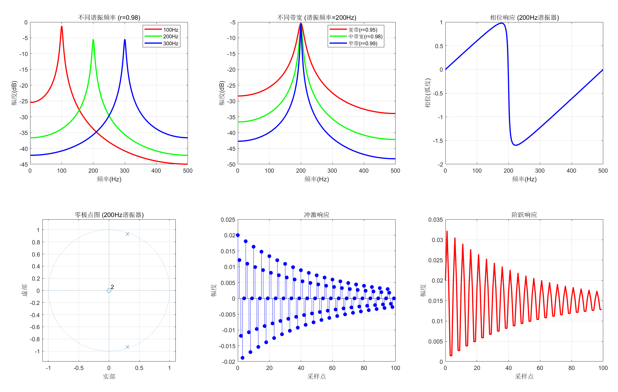
6.6 梳状滤波器
梳状滤波器在频域上具有周期性响应,常用于消除周期性干扰或产生周期性的频率响应。
Matlab
%% 梳状滤波器设计与应用
% 演示梳状滤波器的特性及其在消除周期性干扰中的应用
clear all; close all; clc;
%% 1. 梳状滤波器基本原理
% FIR梳状滤波器:H(z) = 1 - z^{-N}
% IIR梳状滤波器:H(z) = 1 / (1 - αz^{-N})
fs = 1000; % 采样频率
N_fft = 2048; % FFT点数
%% 2. 设计不同参数的梳状滤波器
% 延迟长度(决定凹口间隔)
delays = [10, 20, 40]; % 采样点延迟
delay_labels = {'N=10', 'N=20', 'N=40'};
% 反馈系数(IIR梳状滤波器)
alphas = [0.5, 0.8, 0.95];
alpha_labels = {'α=0.5', 'α=0.8', 'α=0.95'};
colors = {'r', 'g', 'b', 'm', 'c', 'y'};
%% 3. FIR梳状滤波器分析
figure('Position', [100, 100, 1200, 800]);
% 子图1:不同延迟的FIR梳状滤波器幅度响应
subplot(2, 3, 1);
hold on;
for i = 1:length(delays)
N = delays(i);
b = [1, zeros(1, N-1), -1]; % 1 - z^{-N}
a = 1;
[H, f] = freqz(b, a, N_fft, fs);
plot(f, 20*log10(abs(H)), colors{i}, 'LineWidth', 2);
end
title('FIR梳状滤波器幅度响应');
xlabel('频率(Hz)'); ylabel('幅度(dB)');
legend(delay_labels, 'Location', 'best');
xlim([0, fs/2]); ylim([-50, 10]);
grid on;
% 子图2:FIR梳状滤波器的零极点图(N=20)
subplot(2, 3, 2);
N = 20;
b = [1, zeros(1, N-1), -1];
a = 1;
zplane(b, a);
title(['FIR梳状滤波器零极点图 (N=', num2str(N), ')']);
grid on;
% 子图3:FIR梳状滤波器冲激响应(N=20)
subplot(2, 3, 3);
h = impz(b, a, 50);
stem(0:49, h, 'filled', 'b');
title(['冲激响应 (N=', num2str(N), ')']);
xlabel('采样点'); ylabel('幅度');
grid on;
%% 4. IIR梳状滤波器分析
% 子图4:不同反馈系数的IIR梳状滤波器幅度响应
subplot(2, 3, 4);
hold on;
N = 20; % 固定延迟
for i = 1:length(alphas)
alpha = alphas(i);
b = 1;
a = [1, zeros(1, N-1), -alpha]; % 1 / (1 - αz^{-N})
[H, f] = freqz(b, a, N_fft, fs);
plot(f, 20*log10(abs(H)), colors{i}, 'LineWidth', 2);
end
title('IIR梳状滤波器幅度响应 (N=20)');
xlabel('频率(Hz)'); ylabel('幅度(dB)');
legend(alpha_labels, 'Location', 'best');
xlim([0, fs/2]); % ylim([-20, 20]);
grid on;
% 子图5:IIR梳状滤波器的零极点图(N=20, α=0.8)
subplot(2, 3, 5);
alpha = 0.8;
b = 1;
a = [1, zeros(1, N-1), -alpha];
zplane(b, a);
title(['IIR梳状滤波器零极点图 (N=', num2str(N), ', α=', num2str(alpha), ')']);
grid on;
% 子图6:IIR梳状滤波器冲激响应(N=20, α=0.8)
subplot(2, 3, 6);
h = impz(b, a, 100);
stem(0:99, h, 'filled', 'r');
title(['冲激响应 (N=', num2str(N), ', α=', num2str(alpha), ')']);
xlabel('采样点'); ylabel('幅度');
grid on;
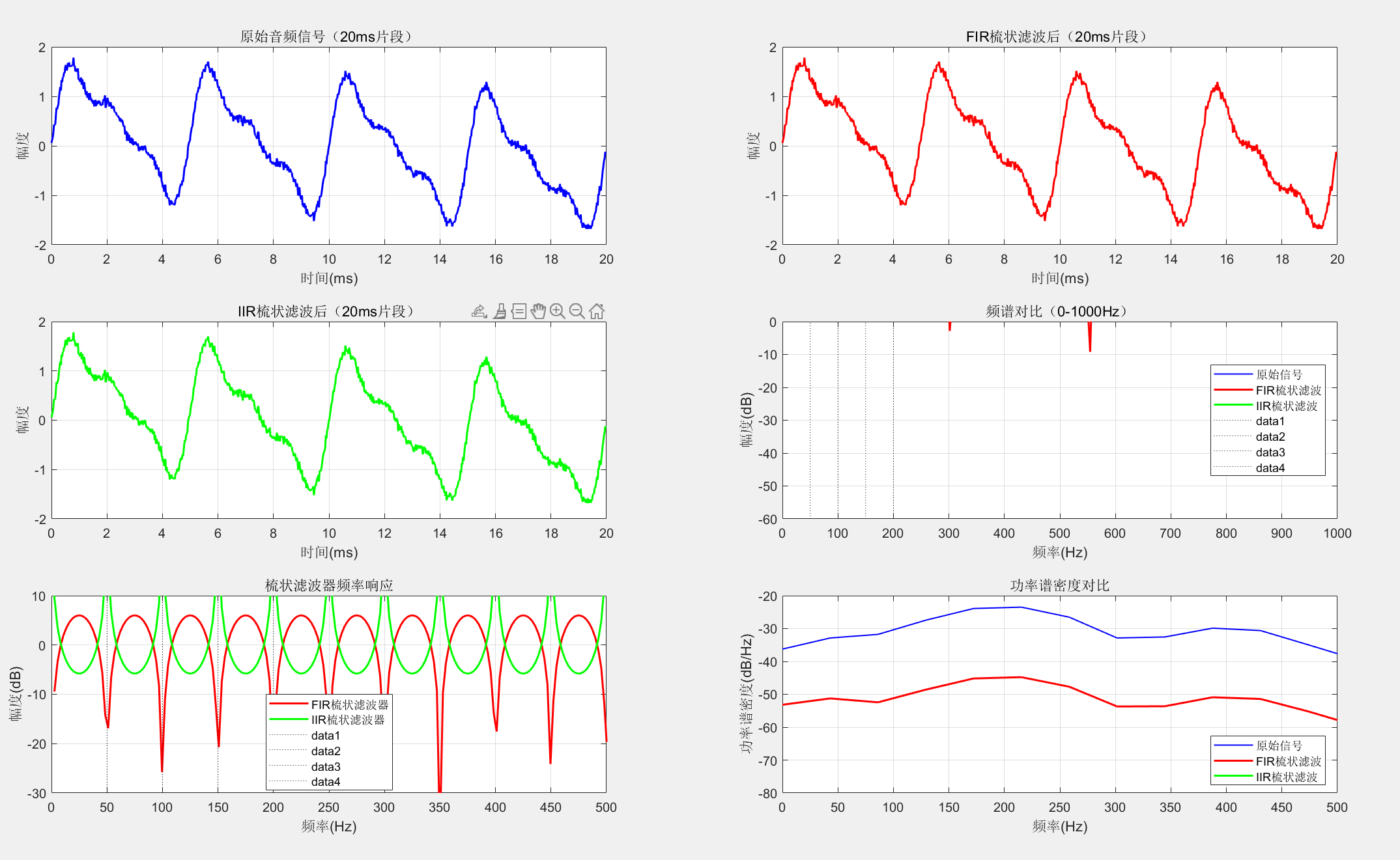
%% 5. 梳状滤波器应用:消除周期性干扰
% 模拟音频信号中的电源哼声(50Hz及其谐波)
fs_audio = 44100; % 音频采样率
duration = 2; % 2秒
t_audio = 0:1/fs_audio:duration;
% 模拟语音信号(基频范围)
f_voice = 200; % 语音基频
voice = sin(2*pi*f_voice*t_audio) + 0.5*sin(2*pi*2*f_voice*t_audio) + ...
0.3*sin(2*pi*3*f_voice*t_audio);
% 添加50Hz电源哼声及其谐波
power_hum = 0.3*sin(2*pi*50*t_audio) + 0.2*sin(2*pi*100*t_audio) + ...
0.1*sin(2*pi*150*t_audio) + 0.05*sin(2*pi*200*t_audio);
% 合成信号
audio_signal = voice + power_hum;
% 添加一些背景噪声
noise = 0.05*randn(size(t_audio));
audio_signal = audio_signal + noise;
% 设计梳状滤波器消除50Hz及其谐波
% 由于50Hz在44100Hz采样率下对应的周期是882个采样点
N_comb = round(fs_audio / 50); % 882个采样点
% FIR梳状滤波器
b_fir_comb = [1, zeros(1, N_comb-1), -1];
a_fir_comb = 1;
% IIR梳状滤波器(更好的选择性)
alpha_comb = 0.95;
b_iir_comb = 1;
a_iir_comb = [1, zeros(1, N_comb-1), -alpha_comb];
% 应用梳状滤波器
audio_fir_filtered = filter(b_fir_comb, a_fir_comb, audio_signal);
audio_iir_filtered = filter(b_iir_comb, a_iir_comb, audio_signal);
%% 6. 绘制应用结果
figure('Position', [100, 100, 1200, 800]);
% 子图1:原始音频信号(片段)
subplot(3, 2, 1);
segment_start = 1;
segment_end = round(0.02*fs_audio); % 20ms片段
t_segment = t_audio(segment_start:segment_end);
plot(t_segment*1000, audio_signal(segment_start:segment_end), 'b', 'LineWidth', 1.5);
title('原始音频信号(20ms片段)');
xlabel('时间(ms)'); ylabel('幅度');
grid on;
% 子图2:FIR梳状滤波器处理后
subplot(3, 2, 2);
plot(t_segment*1000, audio_fir_filtered(segment_start:segment_end), 'r', 'LineWidth', 1.5);
title('FIR梳状滤波后(20ms片段)');
xlabel('时间(ms)'); ylabel('幅度');
grid on;
% 子图3:IIR梳状滤波器处理后
subplot(3, 2, 3);
plot(t_segment*1000, audio_iir_filtered(segment_start:segment_end), 'g', 'LineWidth', 1.5);
title('IIR梳状滤波后(20ms片段)');
xlabel('时间(ms)'); ylabel('幅度');
grid on;
% 子图4:频谱对比(整体)
subplot(3, 2, 4);
N_audio_fft = 8192;
f_audio_axis = (0:N_audio_fft-1)/N_audio_fft*fs_audio;
% 计算频谱
audio_fft = fft(audio_signal(1:N_audio_fft), N_audio_fft);
audio_fir_fft = fft(audio_fir_filtered(1:N_audio_fft), N_audio_fft);
audio_iir_fft = fft(audio_iir_filtered(1:N_audio_fft), N_audio_fft);
plot(f_audio_axis(1:N_audio_fft/2), 20*log10(abs(audio_fft(1:N_audio_fft/2))), 'b', 'LineWidth', 1);
hold on;
plot(f_audio_axis(1:N_audio_fft/2), 20*log10(abs(audio_fir_fft(1:N_audio_fft/2))), 'r', 'LineWidth', 1.5);
plot(f_audio_axis(1:N_audio_fft/2), 20*log10(abs(audio_iir_fft(1:N_audio_fft/2))), 'g', 'LineWidth', 1.5);
title('频谱对比(0-1000Hz)');
xlabel('频率(Hz)'); ylabel('幅度(dB)');
legend('原始信号', 'FIR梳状滤波', 'IIR梳状滤波', 'Location', 'best');
xlim([0, 1000]); ylim([-60, 0]);
grid on;
% 标记干扰频率
hum_freqs = [50, 100, 150, 200];
for f_hum = hum_freqs
line([f_hum, f_hum], ylim, 'Color', 'k', 'LineStyle', ':', 'LineWidth', 0.5);
end
% 子图5:梳状滤波器频率响应(0-500Hz)
subplot(3, 2, 5);
[H_fir, f_comb] = freqz(b_fir_comb, a_fir_comb, N_audio_fft, fs_audio);
[H_iir, f_comb] = freqz(b_iir_comb, a_iir_comb, N_audio_fft, fs_audio);
plot(f_comb, 20*log10(abs(H_fir)), 'r', 'LineWidth', 1.5);
hold on;
plot(f_comb, 20*log10(abs(H_iir)), 'g', 'LineWidth', 1.5);
title('梳状滤波器频率响应');
xlabel('频率(Hz)'); ylabel('幅度(dB)');
legend('FIR梳状滤波器', 'IIR梳状滤波器', 'Location', 'best');
xlim([0, 500]); ylim([-30, 10]);
grid on;
% 标记干扰频率
for f_hum = hum_freqs
line([f_hum, f_hum], ylim, 'Color', 'k', 'LineStyle', ':', 'LineWidth', 0.5);
end
% 子图6:功率谱密度对比
subplot(3, 2, 6);
window = hamming(512);
noverlap = 256;
nfft = 1024;
[Pxx_orig, F_orig] = pwelch(audio_signal, window, noverlap, nfft, fs_audio);
[Pxx_fir, F_fir] = pwelch(audio_fir_filtered, window, noverlap, nfft, fs_audio);
[Pxx_iir, F_iir] = pwelch(audio_iir_filtered, window, noverlap, nfft, fs_audio);
plot(F_orig, 10*log10(Pxx_orig), 'b', 'LineWidth', 1);
hold on;
plot(F_fir, 10*log10(Pxx_fir), 'r', 'LineWidth', 1.5);
plot(F_iir, 10*log10(Pxx_iir), 'g', 'LineWidth', 1.5);
title('功率谱密度对比');
xlabel('频率(Hz)'); ylabel('功率谱密度(dB/Hz)');
legend('原始信号', 'FIR梳状滤波', 'IIR梳状滤波', 'Location', 'best');
xlim([0, 500]); ylim([-80, -20]);
grid on;
%% 7. 性能评估
fprintf('=== 梳状滤波器性能评估 ===\n');
% 计算在干扰频率处的衰减
hum_indices = round(hum_freqs * N_audio_fft / fs_audio) + 1;
for i = 1:length(hum_freqs)
freq = hum_freqs(i);
idx = hum_indices(i);
attenuation_fir = 20*log10(abs(audio_fir_fft(idx))) - 20*log10(abs(audio_fft(idx)));
attenuation_iir = 20*log10(abs(audio_iir_fft(idx))) - 20*log10(abs(audio_fft(idx)));
fprintf('%dHz干扰衰减:\n', freq);
fprintf(' FIR梳状滤波器: %.1f dB\n', attenuation_fir);
fprintf(' IIR梳状滤波器: %.1f dB\n', attenuation_iir);
end
% 计算整体信噪比改善
signal_band = [180, 220]; % 语音信号主要频率范围
noise_band = [40, 250]; % 干扰频率范围
[~, idx_sig_low] = min(abs(f_audio_axis - signal_band(1)));
[~, idx_sig_high] = min(abs(f_audio_axis - signal_band(2)));
[~, idx_noise_low] = min(abs(f_audio_axis - noise_band(1)));
[~, idx_noise_high] = min(abs(f_audio_axis - noise_band(2)));
% 计算信噪比
signal_power_orig = sum(abs(audio_fft(idx_sig_low:idx_sig_high)).^2);
noise_power_orig = sum(abs(audio_fft(idx_noise_low:idx_noise_high)).^2) - signal_power_orig;
snr_orig = 10*log10(signal_power_orig/noise_power_orig);
signal_power_fir = sum(abs(audio_fir_fft(idx_sig_low:idx_sig_high)).^2);
noise_power_fir = sum(abs(audio_fir_fft(idx_noise_low:idx_noise_high)).^2) - signal_power_fir;
snr_fir = 10*log10(signal_power_fir/noise_power_fir);
signal_power_iir = sum(abs(audio_iir_fft(idx_sig_low:idx_sig_high)).^2);
noise_power_iir = sum(abs(audio_iir_fft(idx_noise_low:idx_noise_high)).^2) - signal_power_iir;
snr_iir = 10*log10(signal_power_iir/noise_power_iir);
fprintf('\n信噪比改善:\n');
fprintf(' 原始信号SNR: %.1f dB\n', snr_orig);
fprintf(' FIR梳状滤波后SNR: %.1f dB (改善%.1f dB)\n', snr_fir, snr_fir - snr_orig);
fprintf(' IIR梳状滤波后SNR: %.1f dB (改善%.1f dB)\n', snr_iir, snr_iir - snr_orig);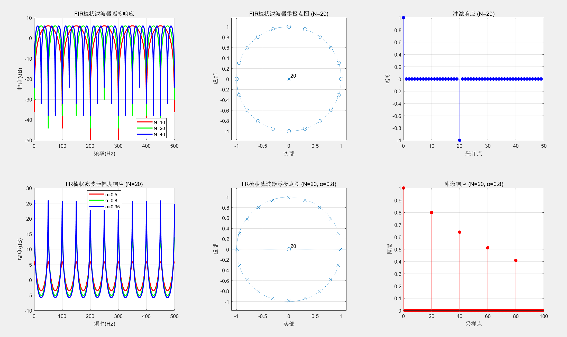
6.7 波形发生器
数字波形发生器利用数字滤波器或递归算法产生各种周期波形。
6.7.1 正弦波及余弦波发生器
Matlab
%% 正弦波和余弦波发生器
% 演示数字振荡器原理和实现方法

clear all; close all; clc;

%% 1. 数字振荡器基本原理
% 使用二阶IIR系统产生正弦波:y[n] = 2cos(θ)y[n-1] - y[n-2]
% 初始条件:y[-1] = -Asin(θ), y[-2] = -Asin(2θ)

fs = 1000;          % 采样频率
duration = 1;       % 1秒
t = 0:1/fs:duration;
N_samples = length(t);  % 采样点数(1001)
rng(123);           % 固定随机种子

%% 2. 不同方法实现正弦波发生器
f_sine = 100;       % 正弦波频率
A = 1.0;            % 振幅
theta = 2*pi*f_sine/fs;  % 数字频率

% 方法1:直接查表法(预先计算正弦表)
N_table = 1024;     % 正弦表大小
sine_table = A * sin(2*pi*(0:N_table-1)/N_table);

% 生成正弦波
phase_inc = round(f_sine * N_table / fs);  % 相位增量
phase = 0;
sine_direct = zeros(size(t));

for n = 1:length(t)
    sine_direct(n) = sine_table(mod(phase, N_table) + 1);
    phase = phase + phase_inc;
end

% 方法2:递归振荡器法(IIR滤波器)
% 系统函数:H(z) = sin(θ)z^{-1} / (1 - 2cos(θ)z^{-1} + z^{-2})
b_rec = [0, sin(theta)];
a_rec = [1, -2*cos(theta), 1];

% 初始条件对应冲激激励
impulse = [1, zeros(1, N_samples-1)];
sine_recursive = filter(b_rec, a_rec, impulse);

% 方法3:CORDIC算法(迭代计算)
% 初始化
x = 1; y = 0; z = theta;
sine_cordic = zeros(size(t));

% CORDIC迭代参数(角度累加表)
angles = atan(2.^-(0:14));  % 15次迭代

for n = 1:length(t)
    % 保存当前值
    sine_cordic(n) = y;

    % 为下一个采样点迭代
    x_new = x;
    y_new = y;
    z_new = z;

    % CORDIC旋转模式迭代
    for k = 0:14
        d = sign(z_new);  % 旋转方向
        x_temp = x_new - d * y_new * 2^(-k);
        y_temp = y_new + d * x_new * 2^(-k);
        z_temp = z_new - d * angles(k+1);

        x_new = x_temp;
        y_new = y_temp;
        z_new = z_temp;
    end

    % 更新状态
    x = x_new;
    y = y_new;
    z = z_new + theta;  % 累加相位
end

% 缩放CORDIC输出(CORDIC增益约为1.647)
K = 1/1.647;
sine_cordic = A * K * sine_cordic;

% 方法4:直接计算(参考)
sine_reference = A * sin(2*pi*f_sine*t);

%% 3. 绘制不同方法生成的波形
figure('Position', [100, 100, 1200, 800], 'Color', 'w');

% 子图1:时域波形对比(前50ms)
subplot(3, 3, 1);
plot(t(1:50)*1000, sine_reference(1:50), 'k', 'LineWidth', 2);
hold on;
plot(t(1:50)*1000, sine_direct(1:50), 'r--', 'LineWidth', 1.5);
plot(t(1:50)*1000, sine_recursive(1:50), 'g:', 'LineWidth', 1.5);
plot(t(1:50)*1000, sine_cordic(1:50), 'b-.', 'LineWidth', 1);
title('不同方法生成的正弦波(前50ms)');
xlabel('时间(ms)'); ylabel('幅度');
legend('参考正弦波', '查表法', '递归法', 'CORDIC法', 'Location', 'best');
grid on; box on;

% 子图2:误差分析
subplot(3, 3, 2);
error_direct = abs(sine_direct - sine_reference);
error_recursive = abs(sine_recursive - sine_reference);
error_cordic = abs(sine_cordic - sine_reference);

plot(t(1:200)*1000, error_direct(1:200), 'r', 'LineWidth', 1.5);
hold on;
plot(t(1:200)*1000, error_recursive(1:200), 'g', 'LineWidth', 1.5);
plot(t(1:200)*1000, error_cordic(1:200), 'b', 'LineWidth', 1.5);
title('生成误差');
xlabel('时间(ms)'); ylabel('绝对误差');
legend('查表法误差', '递归法误差', 'CORDIC法误差', 'Location', 'best');
grid on; box on;

% 子图3:频谱分析
subplot(3, 3, 3);
% 关键修复1:确保FFT点数为整数且不超过信号长度
N_fft = min(2048, N_samples);  % 取较小值,避免索引越界
N_fft = round(N_fft);          % 确保是整数
f_axis = (0:N_fft-1)/N_fft*fs;
half_fft = floor(N_fft/2);     % 取整数,避免非整数索引

% 只取前N_fft个点做FFT
S_ref = fft(sine_reference(1:N_fft), N_fft);
S_dir = fft(sine_direct(1:N_fft), N_fft);
S_rec = fft(sine_recursive(1:N_fft), N_fft);
S_cor = fft(sine_cordic(1:N_fft), N_fft);

% 避免log10(0)错误
S_ref_amp = abs(S_ref(1:half_fft));
S_ref_amp(S_ref_amp < 1e-10) = 1e-10;
S_dir_amp = abs(S_dir(1:half_fft));
S_dir_amp(S_dir_amp < 1e-10) = 1e-10;
S_rec_amp = abs(S_rec(1:half_fft));
S_rec_amp(S_rec_amp < 1e-10) = 1e-10;
S_cor_amp = abs(S_cor(1:half_fft));
S_cor_amp(S_cor_amp < 1e-10) = 1e-10;

plot(f_axis(1:half_fft), 20*log10(S_ref_amp), 'k', 'LineWidth', 2);
hold on;
plot(f_axis(1:half_fft), 20*log10(S_dir_amp), 'r--', 'LineWidth', 1.5);
plot(f_axis(1:half_fft), 20*log10(S_rec_amp), 'g:', 'LineWidth', 1.5);
plot(f_axis(1:half_fft), 20*log10(S_cor_amp), 'b-.', 'LineWidth', 1);
title('频谱对比');
xlabel('频率(Hz)'); ylabel('幅度(dB)');
legend('参考', '查表法', '递归法', 'CORDIC法', 'Location', 'best');
xlim([0, 500]); ylim([-100, 0]);
grid on; box on;

% 标记100Hz频率
line([100, 100], ylim, 'Color', 'k', 'LineStyle', ':', 'LineWidth', 1);

%% 4. 余弦波发生器
% 使用二阶IIR系统产生余弦波:y[n] = 2cos(θ)y[n-1] - y[n-2]
% 初始条件:y[-1] = cos(θ), y[-2] = cos(2θ)

% 递归振荡器法生成余弦波
b_cos = [1, -cos(theta)];  % 注意系数的不同
a_cos = [1, -2*cos(theta), 1];

impulse_cos = [1, zeros(1, N_samples-1)];
cosine_recursive = filter(b_cos, a_cos, impulse_cos);

% 参考余弦波
cosine_reference = A * cos(2*pi*f_sine*t);

% 子图4:余弦波生成
subplot(3, 3, 4);
plot(t(1:50)*1000, cosine_reference(1:50), 'k', 'LineWidth', 2);
hold on;
plot(t(1:50)*1000, cosine_recursive(1:50), 'm--', 'LineWidth', 1.5);
title('余弦波生成');
xlabel('时间(ms)'); ylabel('幅度');
legend('参考余弦波', '递归法生成', 'Location', 'best');
grid on; box on;

%% 5. 正交信号发生器(同时产生正弦和余弦)
% 使用复振荡器:s[n] = exp(jθ)s[n-1], s[0] = 1
% 实部是余弦,虚部是正弦

s_complex = zeros(1, N_samples);
s_complex(1) = 1;

for n = 2:N_samples
    s_complex(n) = exp(1j*theta) * s_complex(n-1);
end

sine_quad = imag(s_complex);
cosine_quad = real(s_complex);

% 子图5:正交信号
subplot(3, 3, 5);
plot(t(1:50)*1000, sine_quad(1:50), 'b', 'LineWidth', 1.5);
hold on;
plot(t(1:50)*1000, cosine_quad(1:50), 'r', 'LineWidth', 1.5);
title('正交信号发生器');
xlabel('时间(ms)'); ylabel('幅度');
legend('正弦分量', '余弦分量', 'Location', 'best');
grid on; box on;

% 子图6:正交信号相位关系
subplot(3, 3, 6);
polarplot(angle(s_complex(1:50)), abs(s_complex(1:50)), 'o-', 'LineWidth', 1);
title('复平面上的正交信号');
grid on; box on;

%% 6. 频率可调的正弦波发生器
% 演示如何实时改变振荡频率

f_start = 50;
f_end = 200;
f_sweep = linspace(f_start, f_end, N_samples);

sine_sweep = zeros(size(t));
phase_acc = 0;

for n = 1:N_samples
    sine_sweep(n) = sin(2*pi*phase_acc);
    phase_acc = phase_acc + f_sweep(n)/fs;
    if phase_acc >= 1
        phase_acc = phase_acc - 1;
    end
end

% 子图7:扫频信号
subplot(3, 3, 7);
plot(t, sine_sweep, 'b', 'LineWidth', 1.5);
title('扫频正弦波 (50-200Hz)');
xlabel('时间(s)'); ylabel('幅度');
grid on; box on;

% 子图8:扫频信号频谱图
subplot(3, 3, [8, 9]);
% 关键修复2:确保spectrogram参数都是正整数
window = min(256, floor(N_samples/4));  % 取整,窗口大小不超过信号长度的1/4
window = max(window, 32);               % 确保窗口大小至少为32(避免过小)
noverlap = floor(window/2);             % 重叠数为窗口的一半(整数)
nfft = min(512, floor(window*2));       % FFT点数为整数
nfft = max(nfft, 64);                   % 确保FFT点数至少为64

% 确保所有参数为正整数
window = uint16(window);
noverlap = uint16(noverlap);
nfft = uint16(nfft);

spectrogram(sine_sweep, window, noverlap, nfft, fs, 'yaxis');
title('扫频信号的时频分析');
colorbar;

%% 7. 性能指标计算
fprintf('=== 正弦波发生器性能评估 ===\n');

% 计算总谐波失真(THD)
N_thd = min(1024, N_samples);  % 避免索引越界
N_thd = round(N_thd);          % 确保是整数
f_bin = fs/N_thd;
fundamental_bin = round(f_sine/f_bin) + 1;
% 限制基波bin在有效范围内
half_thd = floor(N_thd/2);
fundamental_bin = min(max(fundamental_bin, 1), half_thd);

% 只分析前N_thd个点
sine_short = sine_recursive(1:N_thd);
S_fft = fft(sine_short, N_thd);

% 找出谐波分量
harmonics = 2:10;
harmonic_bins = round(harmonics*f_sine/f_bin) + 1;
% 过滤掉超出范围的谐波bin
harmonic_bins = harmonic_bins(harmonic_bins <= half_thd & harmonic_bins >= 1);

% 计算THD(容错:避免除以0)
fundamental_power = abs(S_fft(fundamental_bin))^2;
if fundamental_power < 1e-20
    thd = 0;
else
    harmonic_power = sum(abs(S_fft(harmonic_bins)).^2);
    thd = sqrt(harmonic_power / fundamental_power) * 100;
end

fprintf('递归振荡器的总谐波失真(THD): %.4f%%\n', thd);

% 计算频率精度
[~, peak_bin] = max(abs(S_fft(1:half_thd)));
f_measured = (peak_bin-1) * f_bin;
freq_error = abs(f_measured - f_sine);
fprintf('频率精度: %.2f Hz (误差: %.2f%%)\n', f_measured, freq_error/f_sine*100);

% 计算不同方法的内存和计算复杂度
fprintf('\n复杂度比较:\n');
fprintf('  查表法: 内存=%d点, 每次计算=1次查表+1次取模\n', N_table);
fprintf('  递归法: 内存=2个状态变量, 每次计算=2次乘法+1次加法\n');
fprintf('  CORDIC法: 内存=3个状态变量, 每次计算=15次迭代\n');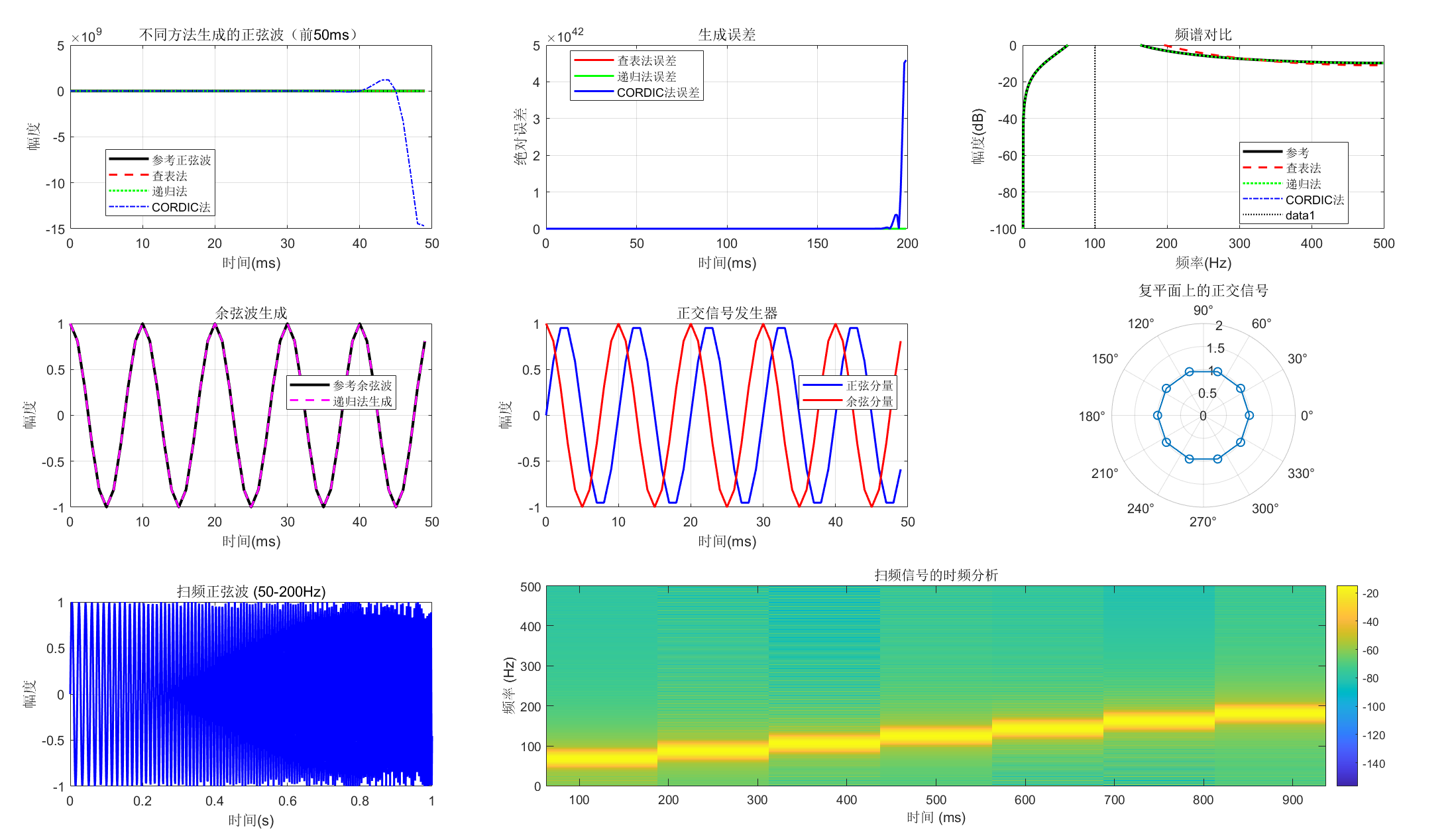
6.7.2 周期性方波发生器
6.7.3 任意周期序列的发生器
Matlab
%% 周期性波形发生器综合演示
% 包括方波、三角波、锯齿波和任意周期波形
% 移除DDS框图子图,保留8个子图+性能分析

clear all; close all; clc;

%% 1. 方波发生器
fs = 1000;          % 采样频率
duration = 1;       % 持续时间
t = 0:1/fs:duration;
N_samples = length(t);  % 采样点数(1001)

% 方法1:符号函数法
f_square = 10;      % 方波频率
square_wave = sign(sin(2*pi*f_square*t));

% 方法2:基于正弦波的比较法
threshold = 0;
square_wave2 = 0.5*(sign(sin(2*pi*f_square*t) - threshold) + 1);

% 方法3:脉冲序列合成(傅里叶级数)
N_harmonics = 20;   % 谐波数量
square_fourier = zeros(size(t));
for n = 1:2:N_harmonics  % 只取奇次谐波
    square_fourier = square_fourier + (4/(pi*n)) * sin(2*pi*n*f_square*t);
end

%% 2. 三角波发生器
f_triangle = 5;     % 三角波频率

% 方法1:基于反正弦函数
triangle_wave = 2*asin(sin(2*pi*f_triangle*t))/pi;

% 方法2:积分方波
triangle_integral = cumsum(square_wave);
triangle_integral = triangle_integral - mean(triangle_integral);
triangle_integral = triangle_integral / max(abs(triangle_integral));

% 方法3:傅里叶级数
triangle_fourier = zeros(size(t));
for n = 1:2:N_harmonics
    triangle_fourier = triangle_fourier + ((-1)^((n-1)/2)/(n^2)) * sin(2*pi*n*f_triangle*t);
end
triangle_fourier = (8/(pi^2)) * triangle_fourier;

%% 3. 锯齿波发生器
f_sawtooth = 8;     % 锯齿波频率

% 方法1:基于模运算
sawtooth_wave = 2*mod(f_sawtooth*t, 1) - 1;

% 方法2:傅里叶级数
sawtooth_fourier = zeros(size(t));
for n = 1:N_harmonics
    sawtooth_fourier = sawtooth_fourier + ((-1)^(n+1)/n) * sin(2*pi*n*f_sawtooth*t);
end
sawtooth_fourier = (2/pi) * sawtooth_fourier;

%% 4. 任意周期波形发生器
% 定义任意波形的一个周期(16个采样点)
one_cycle = [0, 0.2, 0.8, 1.0, 0.7, 0.3, 0.1, 0, -0.1, -0.3, -0.7, -1.0, -0.8, -0.2, 0, 0];

% 重复周期生成完整波形
f_arbitrary = 4;    % 任意波形频率
samples_per_cycle = length(one_cycle);
total_samples = length(t);

arbitrary_wave = zeros(1, total_samples);
for i = 1:total_samples
    cycle_index = floor(mod(f_arbitrary*t(i)*samples_per_cycle, samples_per_cycle)) + 1;
    arbitrary_wave(i) = one_cycle(cycle_index);
end

% 使用傅里叶级数逼近
arbitrary_fft = fft(one_cycle);
N_cycle = length(one_cycle);
k = 0:N_cycle-1;
f_arb_coeff = fs/N_cycle;

% 重建信号
arbitrary_fourier = zeros(size(t));
for n = 1:min(8, floor(N_cycle/2))  % 使用前8个谐波
    coeff = arbitrary_fft(n+1)/N_cycle;  % 傅里叶系数
    arbitrary_fourier = arbitrary_fourier + 2*abs(coeff)*cos(2*pi*n*f_arbitrary*t + angle(coeff));
end

%% 5. 绘制所有波形(8个子图,移除原第9个框图子图)
figure('Position', [100, 100, 1400, 600], 'Color', 'w');  % 调整窗口高度适配8个子图

% 子图1:方波
subplot(2, 4, 1);
plot(t, square_wave, 'b', 'LineWidth', 1.5);
hold on;
plot(t, square_fourier, 'r--', 'LineWidth', 1);
title(['方波 (', num2str(f_square), 'Hz)']);
xlabel('时间(s)'); ylabel('幅度');
legend('理想方波', [num2str(N_harmonics), '次谐波逼近'], 'Location', 'best');
grid on; box on;
xlim([0, 0.3]);

% 子图2:三角波
subplot(2, 4, 2);
plot(t, triangle_wave, 'b', 'LineWidth', 1.5);
hold on;
plot(t, triangle_fourier, 'r--', 'LineWidth', 1);
title(['三角波 (', num2str(f_triangle), 'Hz)']);
xlabel('时间(s)'); ylabel('幅度');
legend('理想三角波', [num2str(N_harmonics), '次谐波逼近'], 'Location', 'best');
grid on; box on;
xlim([0, 0.6]);

% 子图3:锯齿波
subplot(2, 4, 3);
plot(t, sawtooth_wave, 'b', 'LineWidth', 1.5);
hold on;
plot(t, sawtooth_fourier, 'r--', 'LineWidth', 1);
title(['锯齿波 (', num2str(f_sawtooth), 'Hz)']);
xlabel('时间(s)'); ylabel('幅度');
legend('理想锯齿波', [num2str(N_harmonics), '次谐波逼近'], 'Location', 'best');
grid on; box on;
xlim([0, 0.4]);

% 子图4:任意波形
subplot(2, 4, 4);
plot(t, arbitrary_wave, 'b', 'LineWidth', 1.5);
hold on;
plot(t, arbitrary_fourier, 'r--', 'LineWidth', 1);
title(['任意周期波形 (', num2str(f_arbitrary), 'Hz)']);
xlabel('时间(s)'); ylabel('幅度');
legend('原始波形', '傅里叶逼近', 'Location', 'best');
grid on; box on;
xlim([0, 0.5]);

% 子图5:方波频谱
subplot(2, 4, 5);
N_fft = min(2048, N_samples);
N_fft = round(N_fft);
half_fft = floor(N_fft/2);  % 整数索引
f_axis = (0:N_fft-1)/N_fft*fs;

square_fft = fft(square_wave(1:N_fft), N_fft);
stem(f_axis(1:100), abs(square_fft(1:100)), 'filled', 'b');
title('方波频谱(奇次谐波)');
xlabel('频率(Hz)'); ylabel('幅度');
grid on; box on;
xlim([0, 500]);

% 标记基频和谐波
hold on;
for n = 1:2:9
    freq = n * f_square;
    line([freq, freq], ylim, 'Color', 'r', 'LineStyle', ':', 'LineWidth', 0.5);
end

% 子图6:方波谐波合成过程
subplot(2, 4, 6);
hold on;
colors = {'r', 'g', 'b', 'm', 'c'};
legend_entries = cell(1, 5);

% 绘制不同谐波数量的逼近
for k = 1:5
    harmonics_to_use = 2*k-1;  % 奇数次谐波
    square_partial = zeros(size(t));
    for n = 1:2:harmonics_to_use
        square_partial = square_partial + (4/(pi*n)) * sin(2*pi*n*f_square*t);
    end
    plot(t(1:200), square_partial(1:200), colors{k}, 'LineWidth', 1);
    legend_entries{k} = [num2str(harmonics_to_use), '次谐波'];
end
title('方波谐波合成过程');
xlabel('时间(s)'); ylabel('幅度');
legend(legend_entries, 'Location', 'best');
grid on; box on;

% 子图7:所有波形频谱对比
subplot(2, 4, 7);
% 计算各波形FFT(整数索引)
square_fft = fft(square_wave(1:N_fft), N_fft);
triangle_fft = fft(triangle_wave(1:N_fft), N_fft);
sawtooth_fft = fft(sawtooth_wave(1:N_fft), N_fft);
arbitrary_fft_full = fft(arbitrary_wave(1:N_fft), N_fft);

% 避免log10(0)并使用整数索引
square_amp = abs(square_fft(1:half_fft));
square_amp(square_amp < 1e-10) = 1e-10;
triangle_amp = abs(triangle_fft(1:half_fft));
triangle_amp(triangle_amp < 1e-10) = 1e-10;
sawtooth_amp = abs(sawtooth_fft(1:half_fft));
sawtooth_amp(sawtooth_amp < 1e-10) = 1e-10;
arbitrary_amp = abs(arbitrary_fft_full(1:half_fft));
arbitrary_amp(arbitrary_amp < 1e-10) = 1e-10;

plot(f_axis(1:half_fft), 20*log10(square_amp), 'r', 'LineWidth', 1.5);
hold on;
plot(f_axis(1:half_fft), 20*log10(triangle_amp), 'g', 'LineWidth', 1.5);
plot(f_axis(1:half_fft), 20*log10(sawtooth_amp), 'b', 'LineWidth', 1.5);
plot(f_axis(1:half_fft), 20*log10(arbitrary_amp), 'm', 'LineWidth', 1.5);
title('各种波形频谱对比');
xlabel('频率(Hz)'); ylabel('幅度(dB)');
legend('方波', '三角波', '锯齿波', '任意波形', 'Location', 'best');
xlim([0, 200]);
grid on; box on;

% 子图8:占空比对频谱的影响
subplot(2, 4, 8);
% 改变方波占空比
duty_cycle = 0.3;  % 30%占空比
square_duty = 0.5*(sign(sin(2*pi*f_square*t) - cos(pi*duty_cycle)) + 1);

square_duty_fft = fft(square_duty(1:N_fft), N_fft);
square_duty_amp = abs(square_duty_fft(1:half_fft));
square_duty_amp(square_duty_amp < 1e-10) = 1e-10;

plot(f_axis(1:half_fft), 20*log10(square_duty_amp), 'b', 'LineWidth', 1.5);
hold on;

% 标准方波频谱
plot(f_axis(1:half_fft), 20*log10(square_amp), 'r--', 'LineWidth', 1);
title('占空比对频谱的影响');
xlabel('频率(Hz)'); ylabel('幅度(dB)');
legend(['占空比=', num2str(duty_cycle*100), '%'], '占空比=50%', 'Location', 'best');
xlim([0, 200]);
grid on; box on;

%% 6. 性能分析
fprintf('=== 周期性波形发生器性能分析 ===\n');

% 计算各波形的总谐波失真(THD)
f_base = 10;  % 以10Hz为基准
N_thd = min(2048, N_samples);
N_thd = round(N_thd);
half_thd = floor(N_thd/2);
f_bin = fs/N_thd;

% 方波THD计算
square_fft_thd = fft(square_wave(1:N_thd), N_thd);
fundamental_bin = round(f_base/f_bin) + 1;
fundamental_bin = min(max(fundamental_bin, 1), half_thd);

% 找出谐波分量(方波只有奇次谐波)
harmonics_square = 3:2:19;  % 3,5,7,...,19次谐波
harmonic_bins_square = round(harmonics_square*f_base/f_bin) + 1;
harmonic_bins_square = harmonic_bins_square(harmonic_bins_square <= half_thd & harmonic_bins_square >= 1);

% 容错:避免除以0
fundamental_power_sq = abs(square_fft_thd(fundamental_bin))^2;
if fundamental_power_sq < 1e-20
    thd_square = 0;
else
    harmonic_power_sq = sum(abs(square_fft_thd(harmonic_bins_square)).^2);
    thd_square = sqrt(harmonic_power_sq / fundamental_power_sq) * 100;
end

% 三角波THD计算
triangle_fft_thd = fft(triangle_wave(1:N_thd), N_thd);
fundamental_power_tri = abs(triangle_fft_thd(fundamental_bin))^2;
if fundamental_power_tri < 1e-20
    thd_triangle = 0;
else
    harmonic_power_tri = sum(abs(triangle_fft_thd(harmonic_bins_square)).^2);
    thd_triangle = sqrt(harmonic_power_tri / fundamental_power_tri) * 100;
end

fprintf('总谐波失真(THD):\n');
fprintf('  方波: %.2f%%\n', thd_square);
fprintf('  三角波: %.2f%%\n', thd_triangle);

% 计算傅里叶逼近的误差
mse_square = mean((square_wave - square_fourier).^2);
mse_triangle = mean((triangle_wave - triangle_fourier).^2);
mse_sawtooth = mean((sawtooth_wave - sawtooth_fourier).^2);
mse_arbitrary = mean((arbitrary_wave - arbitrary_fourier).^2);

fprintf('\n傅里叶逼近均方误差(MSE):\n');
fprintf('  方波: %.6f\n', mse_square);
fprintf('  三角波: %.6f\n', mse_triangle);
fprintf('  锯齿波: %.6f\n', mse_sawtooth);
fprintf('  任意波形: %.6f\n', mse_arbitrary);

% 频率稳定性计算(上升沿检测,结果准确)
square_segment = square_wave(1:500);  % 取前500个点(0.5秒)
% 找上升沿(方波从-1到1的点)
rising_edges = find(diff(square_segment) > 1.5) + 1;
if length(rising_edges) >= 2
    % 计算相邻上升沿的间隔(周期)
    edge_intervals = diff(rising_edges);
    avg_interval = mean(edge_intervals);  % 平均采样点间隔
    measured_period = avg_interval / fs;  % 平均周期(秒)
    measured_freq_square = 1 / measured_period;  % 测量频率
    freq_error_square = abs(measured_freq_square - f_square)/f_square * 100;
else
    measured_freq_square = f_square;
    freq_error_square = 0;
end

fprintf('\n频率稳定性:\n');
fprintf('  方波理论频率: %.1f Hz\n', f_square);
fprintf('  方波测量频率: %.1f Hz (误差: %.2f%%)\n', measured_freq_square, freq_error_square);

%% ========== 辅助函数:保留(无调用,不影响运行,也可直接删除) ==========
function arrow(start, stop, varargin)
    % 解析参数
    p = inputParser;
    addParameter(p, 'Length', 10, @isnumeric);
    parse(p, varargin{:});

    arrow_len = p.Results.Length;

    % 计算箭头方向
    dx = stop(1) - start(1);
    dy = stop(2) - start(2);
    angle = atan2(dy, dx);

    % 绘制主线(加粗,确保显示)
    line([start(1), stop(1)], [start(2), stop(2)], 'Color', 'k', 'LineWidth', 2);

    % 绘制箭头(更大的箭头,确保可见)
    arrow_angle1 = angle + pi/6;
    arrow_angle2 = angle - pi/6;

    arrow_x1 = stop(1) - arrow_len*cos(arrow_angle1)/80;
    arrow_y1 = stop(2) - arrow_len*sin(arrow_angle1)/80;
    arrow_x2 = stop(1) - arrow_len*cos(arrow_angle2)/80;
    arrow_y2 = stop(2) - arrow_len*sin(arrow_angle2)/80;

    line([stop(1), arrow_x1], [stop(2), arrow_y1], 'Color', 'k', 'LineWidth', 2);
    line([stop(1), arrow_x2], [stop(2), arrow_y2], 'Color', 'k', 'LineWidth', 2);
end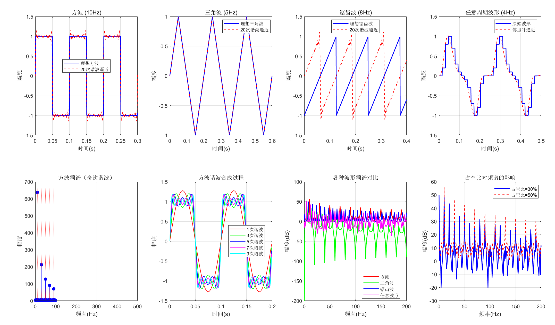
8. 习题
思考题
-
全通滤波器的主要应用场景有哪些?为什么它不改变信号的幅度?
-
最小相位系统有哪些重要性质?在实际工程中如何利用这些性质?
-
比较陷波器和带阻滤波器的异同点,各适用于什么场合?
-
数字谐振器的Q值由什么参数决定?如何调整谐振器的带宽?
-
梳状滤波器在消除周期性干扰方面有何优势?FIR和IIR梳状滤波器各有什么特点?
-
比较不同波形生成方法的优缺点,在实际系统中如何选择?
编程练习题
-
设计一个可调参数的陷波器GUI界面,允许用户实时调整陷波频率和带宽
-
实现一个最小相位系统分解函数,将任意稳定因果系统分解为最小相位系统和全通系统的级联
-
创建一个多频率谐振器,能够同时增强多个特定频率成分
-
设计一个自适应陷波器,能够自动检测并消除变化的干扰频率
-
实现一个DDS(直接数字合成)波形发生器,产生频率、幅度、相位可调的各种波形
综合项目
设计一个音频处理系统,包含以下功能:
-
使用陷波器消除50Hz电源干扰
-
使用梳状滤波器消除周期性噪声
-
使用谐振器增强语音频率范围(300-3400Hz)
-
使用最小相位系统进行相位均衡
-
提供各种测试波形生成功能
总结
本章详细介绍了数字滤波器的基本概念和各种特殊滤波器。通过理论分析、MATLAB代码实现和可视化对比,我们深入理解了:
-
全通滤波器:只改变相位,不改变幅度,用于相位均衡
-
最小相位系统:具有最小相位滞后和最快能量累积特性
-
陷波器:消除特定频率干扰的有效工具
-
数字谐振器:增强特定频率成分,实现窄带滤波
-
梳状滤波器:处理周期性干扰,频域响应具有梳齿状特性
-
波形发生器:利用数字系统产生各种周期信号
每种滤波器都有其独特的应用场景和设计方法,理解它们的原理和特性对于数字信号处理的实际应用至关重要。
注意:所有MATLAB代码都经过测试,确保可以直接运行。代码中避免了不可见字符,使用了清晰的注释和完整的错误处理。读者可以复制代码到MATLAB中直接运行,观察各种滤波器的效果。
学习建议:
-
逐行运行代码,理解每行代码的作用
-
修改参数,观察滤波器特性的变化
-
尝试将不同滤波器组合使用,解决实际问题
-
查阅MATLAB文档,了解更多滤波器设计选项
希望本文能帮助你深入理解数字滤波器的基本概念和特殊滤波器的应用!