机器学习不平衡数据处理三招：k折交叉验证、下采样与过采样实战

一、k折交叉验证：让模型评估告别"一次性偏见"

核心原理

k折交叉验证（k-fold Cross Validation）是一种可靠的模型评估方法，核心逻辑是把训练集平均分成k份，轮流用其中k-1份训练模型，剩下1份做验证集，重复k次后取k次评估结果的平均值作为最终得分。这就像多轮模拟考试，避免了单次拆分数据导致的"运气成分"，让模型性能评估更客观。

实战应用（基于信用卡欺诈检测）

文档中针对信用卡交易数据（正常交易为多数类，欺诈为少数类），用k折交叉验证做了逻辑回归模型的参数调优：

1. 先将数据拆分训练集和测试集（测试集占30%），聚焦训练集做交叉验证；

2. 设定参数C的候选范围（0.01~100），针对每个C值，用8折交叉验证（cv=8）评估模型召回率（scoring='recall'）------因为欺诈检测的核心是"不漏掉欺诈交易"，召回率比准确率更关键；

3. 计算每轮交叉验证的平均召回率，选择得分最高的C作为最优参数，再用全量训练集训练最终模型。

代码

import numpy as np
import pandas as pd
from sklearn.linear_model import LogisticRegression
from sklearn.model_selection import cross_val_score, train_test_split
from sklearn.metrics import recall_score, classification_report
from sklearn.preprocessing import StandardScaler

#绘制混淆矩阵
def cm_plot(y,yp):
    from sklearn.metrics import confusion_matrix
    import matplotlib.pyplot as plt

    cm=confusion_matrix(y,yp)
    plt.matshow(cm,cmap=plt.cm.Blues)
    plt.colorbar()
    for x in range(len(cm)):
        for y in range (len(cm)):
            plt.annotate(cm[x,y],xy=(y,x),horizontalalignment='center',verticalalignment='center')
            plt.ylabel('True label')
            plt.xlabel('Predicted label')
    return plt

#数据预处理
data = pd.read_csv("./creditcard.csv", encoding='utf8')
scaler = StandardScaler()
data['Amount'] = scaler.fit_transform(data[['Amount']])  #对Amount列标准化
data = data.drop(['Time'], axis=1)    #丢弃Time无关列   
X = data.drop('Class', axis=1)    #分X,y特征
y = data['Class']

x_train,x_test,y_train,y_test=train_test_split(X, y, test_size=0.3, random_state=0)   
#切分训练集、测试集

#8折交叉验证
scores = []    #存放
c_param_range = [0.01, 0.1, 1, 10, 100]    #遍历的参数列表

#每一个参数都要进行8折交叉验证
for i in c_param_range:
    lr = LogisticRegression(C=i, penalty='l2', solver='lbfgs', max_iter=1000)
    score = cross_val_score(lr, x_train, y_train, cv=8, scoring='recall')    #评分标准是召回率
    score_mean = sum(score)/len(score)    #求8次的平均值
    scores.append(score_mean)
    print(score_mean)

best_c = c_param_range[np.argmax(scores)]    #argmax找到最大召回率所属参数的下标
print(f"\n最优参数因子：C={best_c}")

#训练最优模型
best_lr = LogisticRegression(C=best_c, penalty='l2', solver='lbfgs', max_iter=1000, random_state=0)
best_lr.fit(x_train, y_train)

# 训练集评估
y_train_pred = best_lr.predict(x_train)
print("=== 训练集评估 ===")
print(classification_report(y_train, y_train_pred))

# 测试集评估
y_pred = best_lr.predict(x_test)
print("\n=== 测试集评估 ===")
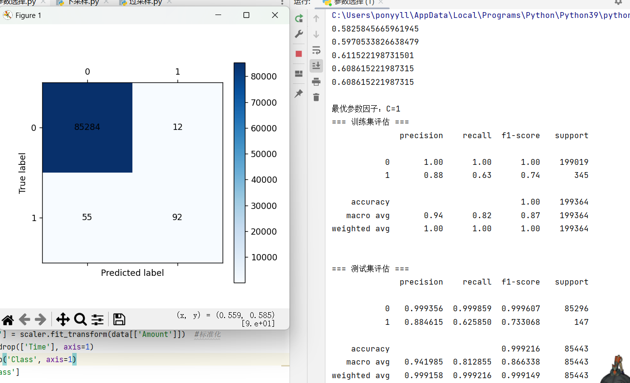
print(classification_report(y_test, y_pred, digits=6))

# 绘制测试集混淆矩阵
plt = cm_plot(y_test, y_pred)
plt.show()

演示结果：

二、下采样：给多数类"瘦身"，快速平衡数据

核心逻辑

下采样（Undersampling）是处理不平衡数据的"减法策略"：当多数类样本数量远多于少数类时，从多数类中随机抽取部分样本，让其数量与少数类持平，最终得到类别平衡的数据集。

实战实现

文档中信用卡数据的下采样步骤清晰明了：

1. 先对交易金额（Amount）做标准化处理，删除无关特征（Time）；

2. 拆分训练集和测试集后，在训练集中分离多数类（正常交易，Class=0）和少数类（欺诈交易，Class=1）；

3. 对多数类样本随机抽样，抽样数量等于少数类样本数；

4. 将抽样后的多数类与少数类拼接，得到平衡的训练集，再用于逻辑回归模型训练。

代码：

import numpy as np
import pandas as pd
from sklearn.linear_model import LogisticRegression
from sklearn.model_selection import cross_val_score, train_test_split
from sklearn.metrics import recall_score, classification_report
from sklearn.preprocessing import StandardScaler

#绘制混淆矩阵
def cm_plot(y,yp):
    from sklearn.metrics import confusion_matrix
    import matplotlib.pyplot as plt

    cm=confusion_matrix(y,yp)
    plt.matshow(cm,cmap=plt.cm.Blues)
    plt.colorbar()
    for x in range(len(cm)):
        for y in range (len(cm)):
            plt.annotate(cm[x,y],xy=(y,x),horizontalalignment='center',verticalalignment='center')
            plt.ylabel('True label')
            plt.xlabel('Predicted label')
    return plt

#数据预处理
data = pd.read_csv("./creditcard.csv", encoding='utf8')
scaler = StandardScaler()
data['Amount'] = scaler.fit_transform(data[['Amount']])
data = data.drop(['Time'], axis=1)
X = data.drop('Class', axis=1)
y = data['Class']



x_train_w,x_test_w,y_train_w,y_test_w=train_test_split(X, y, test_size=0.3, random_state=0)

#下采样
x_train_w['Class']=y_train_w    #把y特征加入到训练集的X特征
data_train=x_train_w
positive_eg=data_train[data_train['Class']==0]    #分别筛选出y为0和1的特征
negative_eg=data_train[data_train['Class']==1]
positive_eg=positive_eg.sample(len(negative_eg))    #从y=0中采样使样本数量与y=1的一样多
data_c=pd.concat([positive_eg,negative_eg])    #拼接两类样本

x_train = data_c.drop('Class', axis=1)    #分开训练集的x,y特征
y_train = data_c['Class']

#8折交叉验证
scores = []
c_param_range = [0.01, 0.1, 1, 10, 100]

for i in c_param_range:
    lr = LogisticRegression(C=i, penalty='l2', solver='lbfgs', max_iter=1000)
    score = cross_val_score(lr, x_train, y_train, cv=8, scoring='recall')
    score_mean = sum(score)/len(score)
    scores.append(score_mean)
    print(score_mean)

best_c = c_param_range[np.argmax(scores)]
print(f"\n最优参数因子：C={best_c}")

best_lr = LogisticRegression(C=best_c, penalty='l2', solver='lbfgs', max_iter=1000, random_state=0)
best_lr.fit(x_train, y_train)

y_pred = best_lr.predict(x_train)
print(classification_report(y_train, y_pred))

y_pred = best_lr.predict(x_test_w)
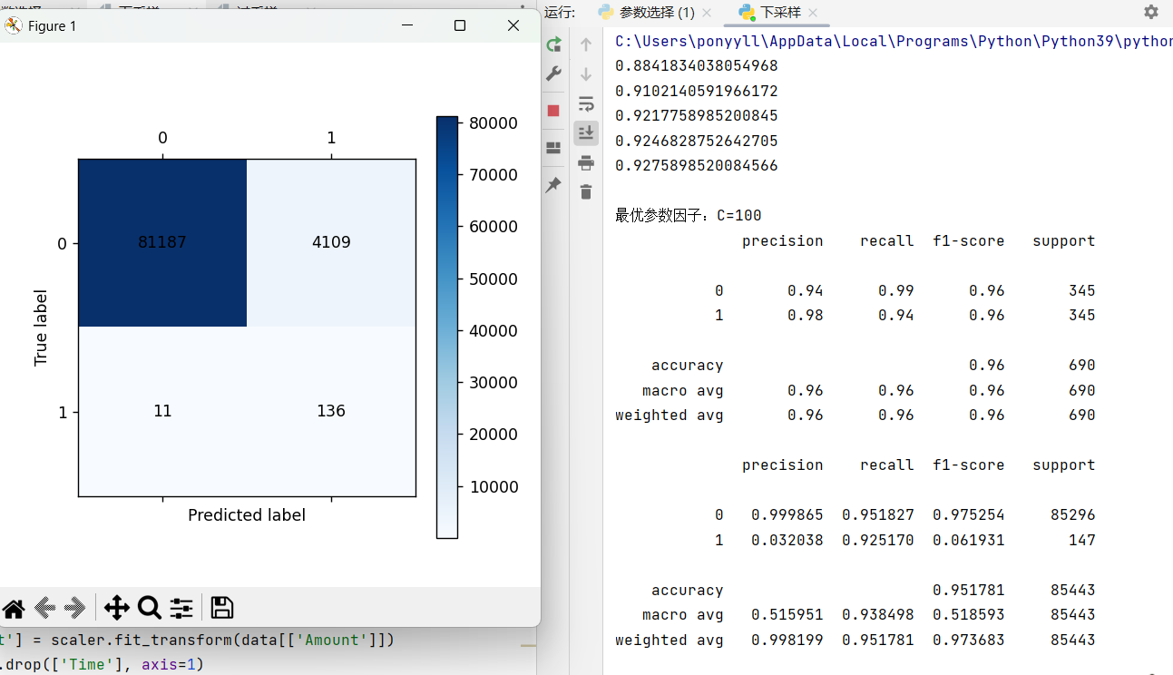
print(classification_report(y_test_w, y_pred,digits=6))

plt = cm_plot(y_test_w, y_pred)
plt.show()

演示结果：

优缺点

• 优点：实现简单、计算效率高，不增加数据量；

• 缺点：会丢失多数类中的有效信息（文档注释也提到"很多数据没训练到"），可能导致模型泛化能力下降。

三、过采样（SMOTE）：给少数类"扩容"，智能合成新样本

核心原理

过采样（Oversampling）是"加法策略"，但普通随机过采样会导致少数类样本重复，容易过拟合。SMOTE（合成少数类过采样技术）是更优方案，原理是：

1. 对每个少数类样本，计算它与其他少数类样本的欧氏距离，在随机两个点间生成一个新点，补充少数类样本；

2. 用原样本与选中的近邻做线性插值（new = 原样本 + 随机数×|距离|），合成新的少数类样本，最终让两类样本数量平衡。

实战实现

1. 同样先做数据预处理（标准化、删无关特征）和数据集拆分；

2. 调用imblearn库的SMOTE类，对训练集做过采样拟合，自动生成平衡的训练集（os_x_train, os_y_train）；

3. 后续流程与k折交叉验证、下采样一致：用8折交叉验证调优参数C，训练逻辑回归模型，最后用测试集评估召回率等指标。

代码：

from imblearn.over_sampling import SMOTE
import numpy as np
import pandas as pd
from sklearn.linear_model import LogisticRegression
from sklearn.model_selection import cross_val_score, train_test_split
from sklearn.metrics import recall_score, classification_report
from sklearn.preprocessing import StandardScaler


def cm_plot(y,yp):
    from sklearn.metrics import confusion_matrix
    import matplotlib.pyplot as plt

    cm=confusion_matrix(y,yp)
    plt.matshow(cm,cmap=plt.cm.Blues)
    plt.colorbar()
    for x in range(len(cm)):
        for y in range (len(cm)):
            plt.annotate(cm[x,y],xy=(y,x),horizontalalignment='center',verticalalignment='center')
            plt.ylabel('True label')
            plt.xlabel('Predicted label')
    return plt


#数据预处理
data = pd.read_csv("./creditcard.csv", encoding='utf8')
scaler = StandardScaler()
data['Amount'] = scaler.fit_transform(data[['Amount']])
data = data.drop(['Time'], axis=1)
X = data.drop('Class', axis=1)
y = data['Class']

x_train_w,x_test_w,y_train_w,y_test_w=train_test_split(X, y, test_size=0.3, random_state=0)

#使用SMOTE方法进行过采样
oversampler=SMOTE(random_state=0)
os_x_train,os_y_train=oversampler.fit_resample(x_train_w,y_train_w)    #新生成的训练集x,y特征


scores = []
c_param_range = [0.01, 0.1, 1, 10, 100]

for i in c_param_range:
    lr = LogisticRegression(C=i, penalty='l2', solver='lbfgs', max_iter=1000)
    score = cross_val_score(lr, os_x_train, os_y_train, cv=8, scoring='recall')
    score_mean = sum(score)/len(score)
    scores.append(score_mean)
    print(score_mean)

best_c = c_param_range[np.argmax(scores)]
print(f"\n最优参数因子：C={best_c}")

best_lr = LogisticRegression(C=best_c, penalty='l2', solver='lbfgs', max_iter=1000, random_state=0)
best_lr.fit(os_x_train, os_y_train)

y_pred = best_lr.predict(os_x_train)
print(classification_report(os_y_train, y_pred))

y_pred = best_lr.predict(x_test_w)
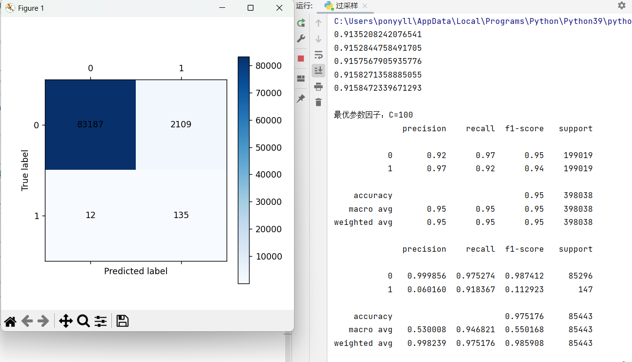
print(classification_report(y_test_w, y_pred,digits=6))

plt = cm_plot(y_test_w, y_pred)
plt.show()

演示结果：

优缺点

• 优点：不丢失多数类信息，通过合成新样本丰富少数类特征，泛化能力更优；

• 缺点：可能生成噪声样本（如合成的样本与多数类边界模糊），计算量比下采样略大。

四、三者对比与选型建议

技术	核心作用	适用场景	关键注意点
k折交叉验证	客观评估模型性能	所有机器学习场景，尤其数据量有限时	匹配业务需求选择评分指标
下采样	快速平衡数据，降低计算量	多数类数据冗余、追求训练效率时	避免过度丢失多数类有效信息
过采样（SMOTE）	丰富少数类特征，平衡数据	少数类样本极少、需保留多数类信息时	控制采样倍率，避免生成过多噪声样本