机器学习算法原理与实践-入门(十一):基于PyTorch的房价预测实战
在前面的文章中,我们已经系统学习了PyTorch框架的基本使用和线性回归的实现原理。今天,我们将把这些知识应用到实际项目中------基于PyTorch框架的房价预测。这是一个完整的机器学习项目,涵盖了从数据预处理到模型训练再到结果可视化的全流程。
一、项目背景与目标
1.1 房价预测的意义
房价预测是机器学习在房地产领域的经典应用场景。通过分析影响房价的各种因素(如地理位置、房屋年龄、交通便利性等),我们可以构建模型来预测房屋单位面积价格,这对房地产投资、市场分析和个人购房决策都具有重要参考价值。
1.2 项目目标
本项目将使用台湾新北市的房地产交易数据,构建一个线性回归模型,预测房屋单位面积的价格。通过这个项目,你将学会:
- 如何准备和处理真实的房地产数据
- 如何使用PyTorch构建完整的机器学习流水线
- 如何评估回归模型的性能
- 如何可视化模型的预测结果
二、数据准备与预处理
2.1 数据集介绍
我们使用的数据集包含以下特征:
- X1: 交易日期
- X2: 房屋年龄
- X3: 到最近地铁站的距离
- X4: 周边便利店数量
- X5: 纬度
- X6: 经度
- Y: 房屋单位面积价格(目标变量)
2.2 关键技术点
One-Hot编码:对于便利店数量这类离散特征,我们使用独热编码将其转换为二进制特征向量,这样模型可以更好地理解这类分类特征。
数据标准化:使用StandardScaler将所有特征标准化到均值为0、方差为1的分布,这有助于提高模型训练的稳定性和收敛速度。
三、完整代码实现
python
import pandas as pd
from sklearn.model_selection import train_test_split
from sklearn.utils import shuffle
from sklearn.preprocessing import StandardScaler
import torch
import torch.nn as nn
import torch.optim as optim
import matplotlib.pyplot as plt
# 1. 读取数据集
data = pd.read_excel('../dataset/Real estate valuation data set.xlsx')
print("数据预览:")
print(data.head())
# 2. 数据预处理
# 对便利店数量进行One-Hot编码
data = pd.get_dummies(data, columns=['X4 number of convenience stores'])
# 提取特征和目标变量
feature_columns = ['X1 transaction date', 'X2 house age',
'X3 distance to the nearest MRT station', 'X5 latitude', 'X6 longitude']
# 添加One-Hot编码后的便利店特征
store_columns = [col for col in data.columns if 'X4 number of convenience stores_' in col]
feature_columns.extend(store_columns)
X = data[feature_columns]
y = data['Y house price of unit area']
# 3. 数据集划分
# 打乱数据并划分训练集和测试集
train_ratio = 0.8
X, y = shuffle(X, y)
X_train = X[:int(train_ratio * len(data))]
X_test = X[int((train_ratio) * len(data)):]
y_train = y[:int(train_ratio * len(data))]
y_test = y[int((train_ratio) * len(data)):]
# 4. 数据标准化
scaler = StandardScaler()
X_train_scaled = scaler.fit_transform(X_train)
X_test_scaled = scaler.transform(X_test)
# 5. 转换为PyTorch Tensor
X_train_tensor = torch.tensor(X_train_scaled, dtype=torch.float32)
y_train_tensor = torch.tensor(y_train.values, dtype=torch.float32).view(-1, 1)
X_test_tensor = torch.tensor(X_test_scaled, dtype=torch.float32)
y_test_tensor = torch.tensor(y_test.values, dtype=torch.float32).view(-1, 1)
# 6. 定义线性回归模型
class LinearRegressionModel(nn.Module):
def __init__(self, input_size):
super(LinearRegressionModel, self).__init__()
self.linear = nn.Linear(input_size, 1)
def forward(self, x):
return self.linear(x)
# 7. 模型初始化
model = LinearRegressionModel(X_train_tensor.shape[1])
criterion = nn.MSELoss()
optimizer = optim.Adam(model.parameters(), lr=0.1)
# 8. 模型训练
num_epochs = 1000
train_losses = []
for epoch in range(num_epochs):
model.train()
optimizer.zero_grad()
# 前向传播
predictions = model(X_train_tensor)
loss = criterion(predictions, y_train_tensor)
# 反向传播与优化
loss.backward()
optimizer.step()
# 记录损失
train_losses.append(loss.item())
# 打印训练进度
if (epoch + 1) % 100 == 0:
print(f'Epoch [{epoch + 1}/{num_epochs}], Loss: {loss.item():.4f}')
# 9. 模型评估
model.eval()
with torch.no_grad():
test_predictions = model(X_test_tensor)
test_loss = criterion(test_predictions, y_test_tensor)
print(f'\n测试集损失: {test_loss.item():.4f}')
# 10. 结果可视化
# 转换为numpy数组用于绘图
predictions_np = test_predictions.numpy()
y_test_np = y_test_tensor.numpy()
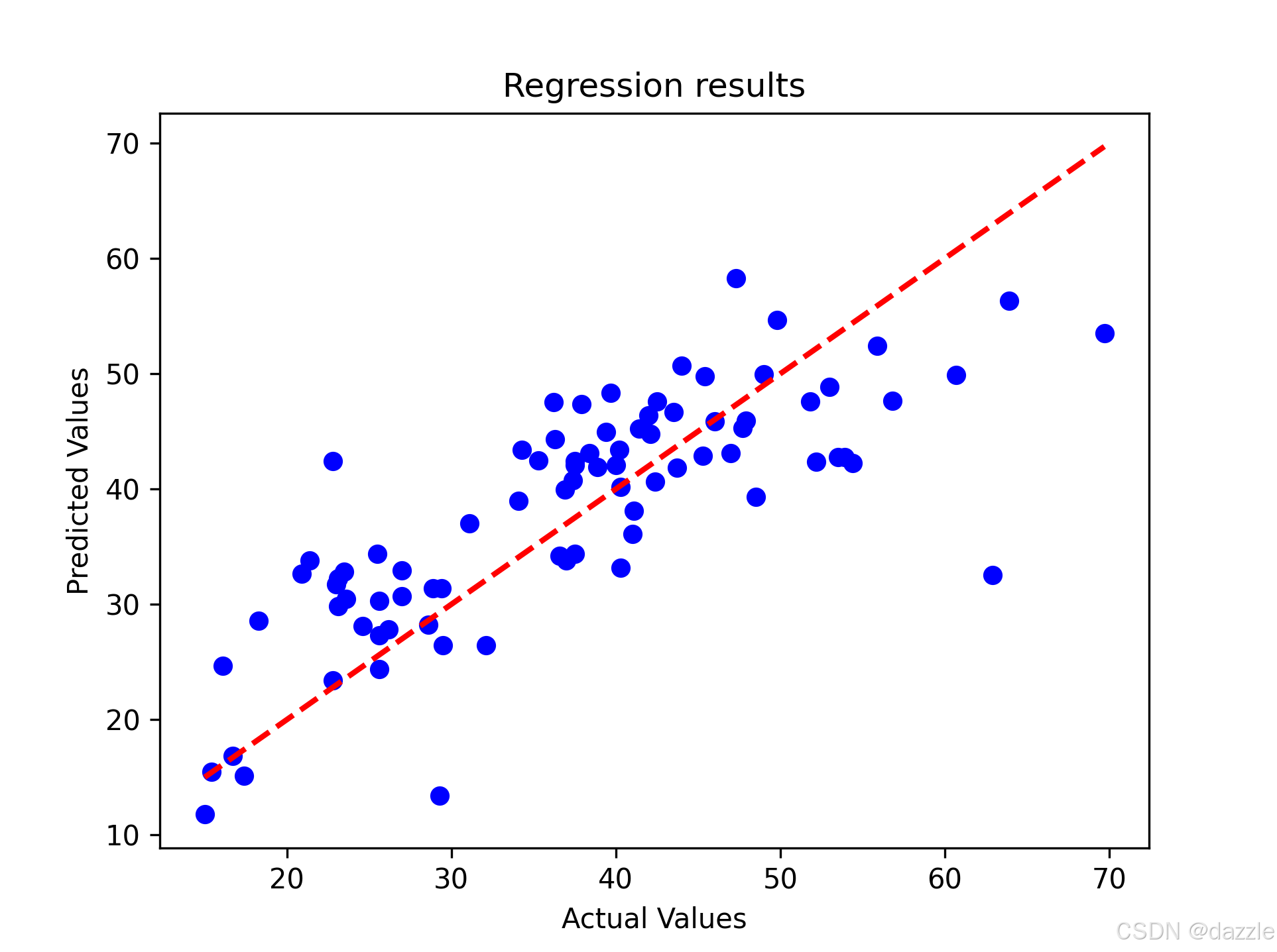
# 图1:预测值 vs 真实值散点图
plt.figure(figsize=(12, 5))
plt.subplot(1, 2, 1)
plt.scatter(y_test_np, predictions_np, alpha=0.6, color='blue')
plt.plot([y_test_np.min(), y_test_np.max()],
[y_test_np.min(), y_test_np.max()],
'r--', linewidth=2, label='完美预测线')
plt.xlabel('实际房价')
plt.ylabel('预测房价')
plt.title('预测值与真实值对比')
plt.legend()
plt.grid(True, alpha=0.3)
# 图2:训练损失曲线
plt.subplot(1, 2, 2)
plt.plot(range(num_epochs), train_losses, 'b-', linewidth=1.5)
plt.xlabel('训练轮次')
plt.ylabel('损失值')
plt.title('训练损失变化曲线')
plt.grid(True, alpha=0.3)
plt.tight_layout()
plt.show()
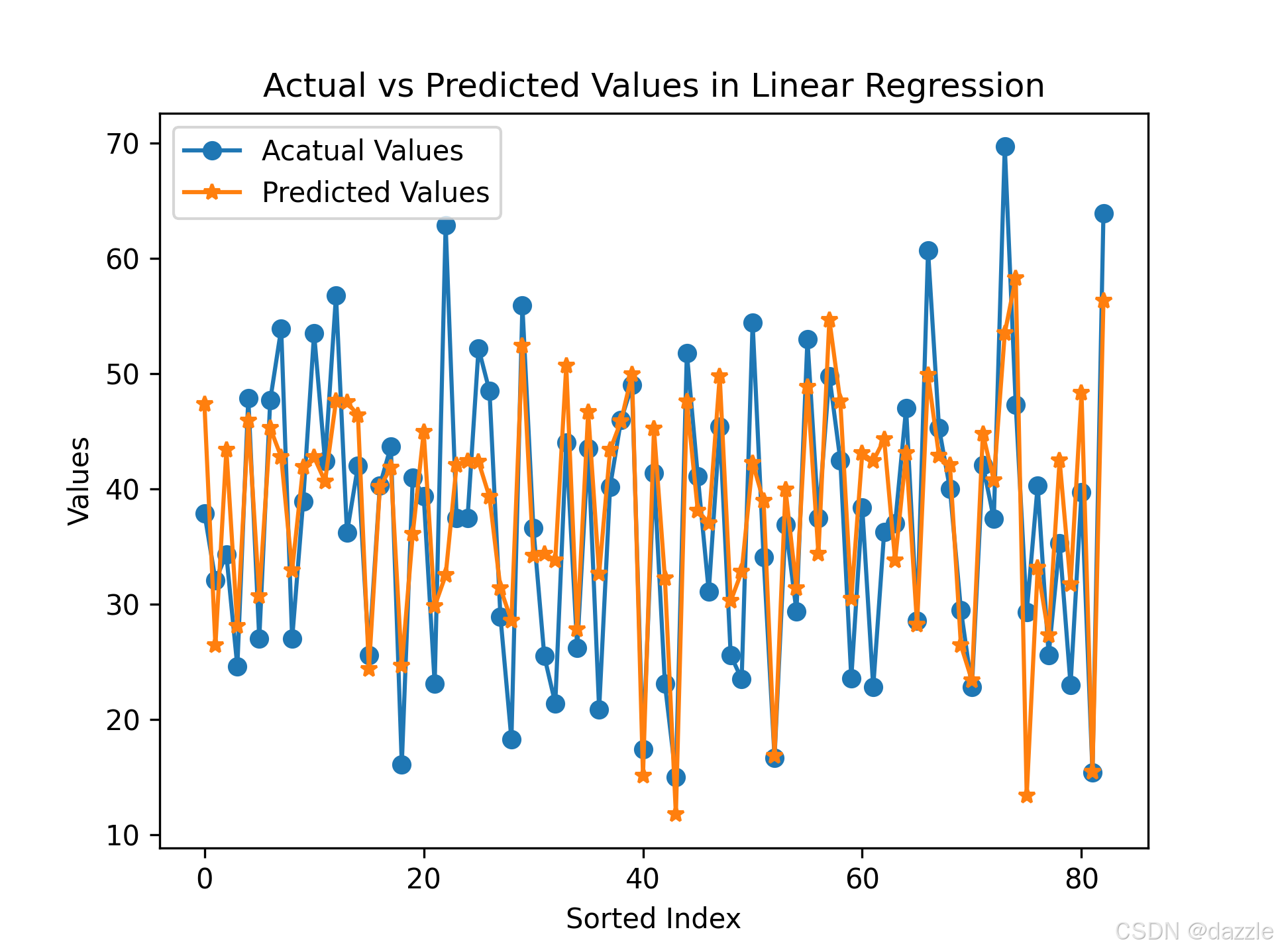
# 11. 预测结果排序展示
sorted_indices = X_test.index.argsort()
y_test_sorted = y_test.iloc[sorted_indices]
y_pred_sorted = pd.Series(predictions_np.squeeze()).iloc[sorted_indices]
plt.figure(figsize=(10, 6))
plt.plot(y_test_sorted.values, 'o-', label='实际值', markersize=6)
plt.plot(y_pred_sorted.values, 's-', label='预测值', markersize=4)
plt.xlabel('排序后的样本索引')
plt.ylabel('房价')
plt.title('实际值与预测值对比(排序后)')
plt.legend()
plt.grid(True, alpha=0.3)
plt.show()四、代码关键点讲解
4.1 数据预处理策略
python
# One-Hot编码处理离散特征
data = pd.get_dummies(data, columns=['X4 number of convenience stores'])为什么需要One-Hot编码:便利店数量(0, 1, 2, ...)虽然看起来是数值,但实际上表示的是分类信息。直接作为连续数值处理会让模型误认为"10家便利店"是"5家便利店"的两倍,而实际上这只是类别的不同。
4.2 数据标准化的重要性
python
scaler = StandardScaler()
X_train_scaled = scaler.fit_transform(X_train)
X_test_scaled = scaler.transform(X_test)标准化原理:将每个特征减去其均值,然后除以其标准差。这样处理后,所有特征都处于同一数量级,避免某些特征因为数值较大而对模型产生过大的影响。
4.3 模型定义
python
class LinearRegressionModel(nn.Module):
    def __init__(self, input_size):
        super(LinearRegressionModel, self).__init__()
        self.linear = nn.Linear(input_size, 1)

    def forward(self, x):
        return self.linear(x)
nn.Linear层 :这是PyTorch中的全连接层,实现了线性变换 y=xAT+by = xA^T + by=xAT+b。其中input_size是输入特征的维度,1是输出维度(单值预测)。
4.4 训练循环的核心逻辑
python
for epoch in range(num_epochs):
    model.train()  # 设置训练模式
    optimizer.zero_grad()  # 清空梯度

    # 前向传播
    predictions = model(X_train_tensor)
    loss = criterion(predictions, y_train_tensor)

    # 反向传播
    loss.backward()
optimizer.step() # 更新参数训练三部曲:
- 前向传播:计算预测值和损失
- 反向传播:计算损失对参数的梯度
- 参数更新:根据梯度调整参数值
4.5 评估模式的使用
python
model.eval()
with torch.no_grad():
    test_predictions = model(X_test_tensor)
model.eval() :将模型设置为评估模式,这会影响某些层的行为(如Dropout、BatchNorm等)。
torch.no_grad():关闭梯度计算,节省内存并提高推理速度。
五、结果分析与模型评估
5.1 损失函数分析
我们使用均方误差(MSE)作为损失函数:
MSE=1n∑i=1n(yi−y^i)2 MSE = \frac{1}{n} \sum_{i=1}^{n} (y_i - \hat{y}_i)^2 MSE=n1i=1∑n(yi−y^i)2
MSE对较大的误差给予更高的惩罚,这符合我们对房价预测的精度要求。
5.2 可视化解读
散点图分析:理想情况下,所有的点都应该落在红色对角线上。点的分布越接近对角线,说明模型的预测越准确。
损失曲线分析:训练损失应该随着训练轮次的增加而逐渐下降并趋于稳定。如果损失曲线震荡剧烈,可能需要降低学习率;如果下降太慢,可能需要增加学习率。
下一篇预告
在掌握了基于PyTorch的线性回归实战后,我们将进入更加实用的项目:
机器学习算法原理与实践-入门(十二):基于Pytorch的鲍鱼年龄预测预测
我们将使用scikit-learn框架解决一个经典的分类问题,学习如何处理时间序列数据、如何选择不同的分类算法,以及如何评估分类模型的性能。