CHO细胞培养中高乳酸与低产量的模式识别与分析

Process Variability Source Analysis for a Multi-step Bio-process

Mario R. Eden, Marianthi Ierapetritou and Gavin P. Towler (Editors) Proceedings of the 13 th

International Symposium on Process Systems Engineering -- PSE 2018

July 1-5, 2018, San Diego, California, USA © 2018 Elsevier B.V. All rights reserved.

https://doi.org/10.1016/B978-0-444-64241-7.50411-0

目录

一、问题背景与目标

二、业务侧结论

[2.1 高乳酸问题不是"一种"原因，至少存在4类不同机制](#2.1 高乳酸问题不是“一种”原因，至少存在4类不同机制)

[2.2 第2类高乳酸的主要根因指向接种阶段，且与两项可调控参数强相关](#2.2 第2类高乳酸的主要根因指向接种阶段，且与两项可调控参数强相关)

[2.3 可以在生产前预测第2类高乳酸风险，实现早期干预](#2.3 可以在生产前预测第2类高乳酸风险，实现早期干预)

[2.4 不同高乳酸聚类在细胞体积（PCV） 模式上存在显著差异](#2.4 不同高乳酸聚类在细胞体积（PCV） 模式上存在显著差异)

[2.5 未来可拓展的工艺数据采集建议（来自文章展望）](#2.5 未来可拓展的工艺数据采集建议（来自文章展望）)

[2.6 总结：业务侧可执行的3条核心建议](#2.6 总结：业务侧可执行的3条核心建议)

Lac根因分析流程

[1. 适用范围](#1. 适用范围)

[2. 输入数据要求](#2. 输入数据要求)

[3. 软件与工具](#3. 软件与工具)

[4. 分析步骤](#4. 分析步骤)

步骤1：数据预处理

步骤2：数据展开（生产阶段数据）

步骤3：PCA监控模型（基于低乳酸批次）

步骤4：高乳酸批次的层次聚类

步骤5：接种阶段特征筛选与降维

步骤6：SVM分类模型训练与评估

步骤7：根因识别与可视化

[5. 注意事项](#5. 注意事项)

[6. DEMO.py](#6. DEMO.py)

[7. 附录：历史研究贡献与局限](#7. 附录：历史研究贡献与局限)

---

一、问题背景与目标

• 背景 ：在CHO细胞生产单克隆抗体的多步批次过程中，高乳酸 常与低产量相关，是影响工艺稳定性和产品质量的关键因素。

• 挑战：传统基于代谢机制的方法难以应用于大规模生产，因为缺少关键代谢物浓度数据。

• 目标 ：利用历史数据挖掘高乳酸的根本原因 ，并实现在早期阶段（接种阶段） 的预测与干预。

二、业务侧结论

2.1 高乳酸问题不是"一种"原因，至少存在4类不同机制

结论 ：

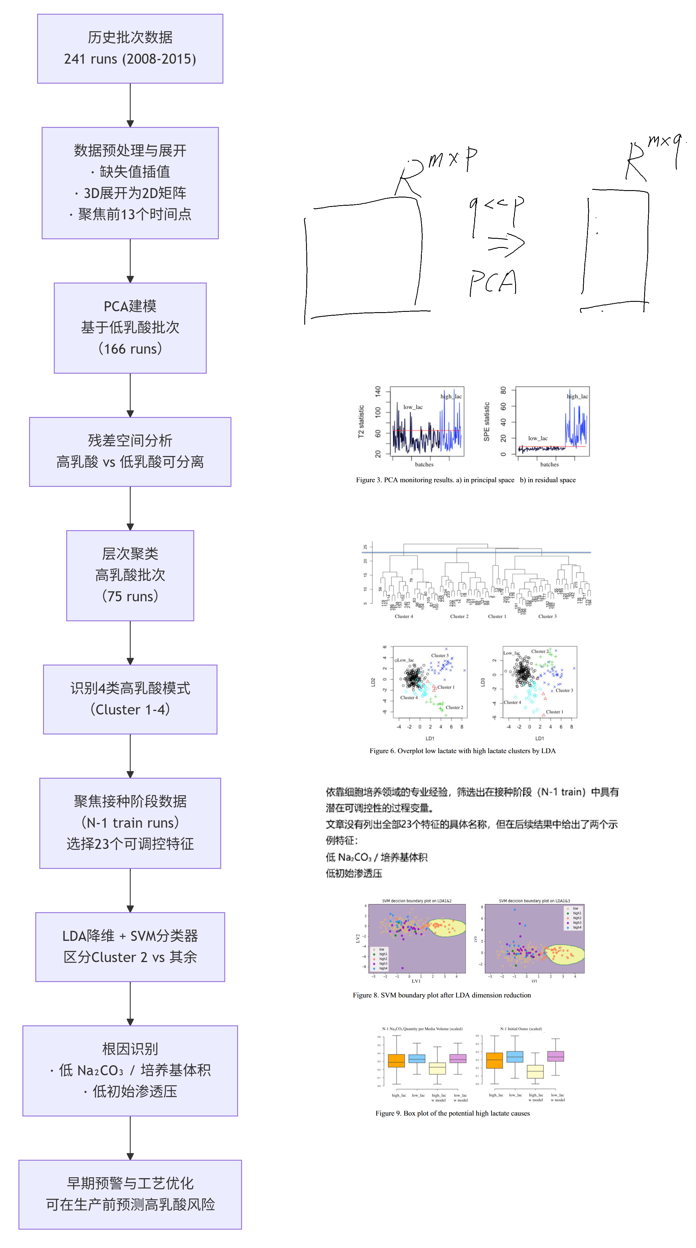
通过对241批生产数据的无监督聚类分析，高乳酸（低性能）批次可以被划分为 4个不同的子类，每个子类在关键生理参数（如PCV、代谢物）上表现出不同的演变模式。

按照我以往项目经验，有以下几种（第二行第一个是通过控糖来抑制lac翘尾）。注：与文中定义第几类的顺序不一样。

• 不要试图用一个"通用低乳酸方案"解决所有高乳酸批次。

• 建议针对每一类高乳酸设计独立的根因排查实验（例如：某类重点看接种条件，其他类可能涉及其他阶段或原料差异）。

---

2.2 第2类高乳酸的主要根因指向接种阶段，且与两项可调控参数强相关

结论：

• 第2类高乳酸（约占部分高乳酸批次）可以在接种（N-1 train）阶段被提前识别。

• 关键驱动因素是：

  • ✅ 低 Na₂CO₃ / 培养基体积（即碳酸钠添加量偏低）

  • ✅ 低初始渗透压

建议：

• 在接种阶段严格监控并优化这两个参数：

  • 适当提高Na₂CO₃添加量（注意控制pH冲击）

  • 提高初始渗透压至合适范围（可通过补加NaCl或调整培养基配方）

• 建议开展DOE实验，在N-1阶段验证这两个参数的调整对生产阶段乳酸积累的影响。

---

2.3 可以在生产前预测第2类高乳酸风险，实现早期干预

结论 ：

使用接种阶段的23个可调节特征 + LDA降维 + SVM分类器，可以提前预测第2类高乳酸，模型性能：

• 误报率（Type I error）仅 2.3%

• 漏报率（Type II error）为 20.6%

建议：

• 可将该模型部署为工艺早期预警工具：在接种阶段结束后即可输出"是否属于第2类高乳酸高风险批次"。

• 对于高风险批次，可提前采取干预措施（如调整补料策略、温度控制、培养基优化）。

• 漏报率仍较高，建议结合其他指标（如PCV变化趋势）做综合判断，而非完全依赖模型。

---

2.4 不同高乳酸聚类在细胞体积（PCV） 模式上存在显著差异

结论 ：

热图分析显示，第2类高乳酸的PCV演变模式与其他类明显不同（例如早期PCV偏低或上升过慢）。

建议：

• 将PCV曲线形态作为辅助诊断指标。

• 对于PCV模式类似第2类的批次，提前关注接种阶段渗透压和Na₂CO₃。

• 对于其他PCV模式的高乳酸批次，需另外设计实验（如代谢物分析、培养基批次差异）。

---

2.5 未来可拓展的工艺数据采集建议（来自文章展望）

结论 ：

目前仅分析了接种阶段和生产阶段数据，但高乳酸的其他聚类可能关联到更早期的细胞解冻数据 或原材料（培养基/补料）批次信息。

建议：

• 建议工艺团队系统记录并共享以下数据给算法团队：

  • 细胞解冻日期、活率、密度

  • 培养基/补料的批次号、生产厂家、储存时间

  • 接种前的细胞传代历史

• 这些数据可能解释目前尚无法归因的第1、3、4类高乳酸原因。

---

2.6 总结：业务侧可执行的3条核心建议

序号	核心建议	对应聚类	可行措施
1	接种阶段提高Na₂CO₃添加量 和初始渗透压	第2类	调整培养基配方或补料策略
2	部署早期SVM预警模型，识别第2类高风险批次	第2类	接种结束后运行模型，提前干预
3	对不同高乳酸类型分别设计根因实验，不要统一处理	全部4类	分类汇总历史批次，设计针对性DOE

Lac根因分析流程

1. 适用范围

本文适用于CHO细胞培养生产单克隆抗体的多步骤批次工艺，基于历史生产数据（含生产阶段在线/离线测量、接种阶段数据、培养基制备数据）进行：

• 高乳酸与低乳酸批次的区分

• 高乳酸批次的隐藏模式识别聚类

• 接种阶段早期预测模型建立

• 潜在可调控根因识别

2. 输入数据要求

数据类型	说明
生产阶段数据（intra-batch）	每个批次多个特征（如PCV、乳酸、葡萄糖等），每天采样2次，共23个时间点
接种阶段数据（N-1 train）	每个批次初始状态、离线测量、培养基制备相关特征（至少23个选定特征）
批次标签	最终乳酸浓度实测值，用于归一化及分类

数据范围：至少包含2008-2015年间的历史批次，建议不少于200批。

数据模板参考如下：

3. 软件与工具

• Python 3.8+ 或 MATLAB R2018b+

• 必需库：numpy, pandas, scikit-learn, matplotlib, seaborn

4. 分析步骤

import numpy as np
import pandas as pd
from sklearn.preprocessing import StandardScaler
from sklearn.decomposition import PCA
from sklearn.cluster import AgglomerativeClustering
from sklearn.discriminant_analysis import LinearDiscriminantAnalysis
from sklearn.svm import SVC
from scipy.cluster.hierarchy import linkage, dendrogram, fcluster
from scipy.stats import f, chi2
import matplotlib.pyplot as plt
from typing import Tuple, Optional, Dict, Any

步骤1：数据预处理

1. 缺失值处理 ：对每个特征的时间序列，采用局部线性插值填补缺失点。

2. 时间点对齐：确保每个批次具有相同的采样时间点（23个点）。

3. 截取关键时间窗口：仅保留前13个时间点（高乳酸不可逆累积发生前的阶段）。

4. 乳酸归一化：

   • 计算所有批次最终乳酸浓度的最小值 Lmin⁡和最大值 Lmax⁡。

   • 归一化值 Lnorm=（L−Lmin）/（⁡Lmax⁡−Lmin​​）。

   • 分类阈值：Lnorm>0.4 为高乳酸批次（低性能），否则为低乳酸批次（高性能）。

def preprocess_and_normalize_lactate(
    lactate_final: np.ndarray,
    threshold: float = 0.4
) -> Tuple[np.ndarray, np.ndarray]:
    """
    对最终乳酸浓度进行归一化，并根据阈值划分高/低乳酸批次。

    Parameters
    ----------
    lactate_final : np.ndarray, shape (n_batches,)
        每个批次的最终乳酸浓度实测值。
    threshold : float, default=0.4
        归一化后的乳酸阈值，大于该值为高乳酸（低性能），否则为低乳酸（高性能）。

    Returns
    -------
    lactate_norm : np.ndarray, shape (n_batches,)
        归一化后的乳酸浓度，范围 [0, 1]。
    high_lactate_mask : np.ndarray, shape (n_batches,), dtype=bool
        True 表示高乳酸批次，False 表示低乳酸批次。
    """
    L_min = np.min(lactate_final)
    L_max = np.max(lactate_final)
    lactate_norm = (lactate_final - L_min) / (L_max - L_min)
    high_lactate_mask = lactate_norm > threshold
    return lactate_norm, high_lactate_mask

步骤2：数据展开（生产阶段数据）

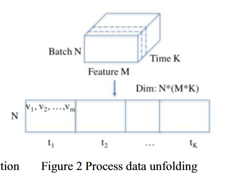
• 原始数据形状：N 批次 × M 特征 × K 时间点（K=13）

• 展开为2D矩阵：每行对应一个批次，每列对应"某一特征在某一时间点"的值，总列数为 M×K。

• 示例：若 M=10 个特征，K=13，则展开后为 N×130 矩阵。

def unfold_3d_to_2d(
    data_3d: np.ndarray,
) -> np.ndarray:
    """
    将三维批次数据 (N, M, K) 展开为二维矩阵 (N, M*K)。

    Parameters
    ----------
    data_3d : np.ndarray, shape (n_batches, n_features, n_timepoints)
        三维原始数据：批次 × 特征 × 时间点。

    Returns
    -------
    data_2d : np.ndarray, shape (n_batches, n_features * n_timepoints)
        展开后的二维矩阵，每列对应一个特征在某个时间点的值。
    """
    n_batches, n_features, n_timepoints = data_3d.shape
    return data_3d.reshape(n_batches, n_features * n_timepoints)

步骤3：PCA监控模型（基于低乳酸批次）

1. 训练数据：所有低乳酸批次（166批）的展开矩阵。

2. PCA拟合：

   • 数据中心化（减去均值），是否缩放取决于特征单位，建议自动缩放（标准化）。

   • 选择主成分数（PCs），使得累计方差解释率 ≥ 95%。【注：按照我的项目经验，基本上前3个主成分的累计方差解释率只有50%左右】

3. 计算控制限：

   • T2 控制限：基于F分布（Qin 2003方法）。

   • SPE（Q统计量）控制限：基于卡方分布加权。

4. 对所有批次（高+低乳酸）计算：

   • 在PCA模型下投影，得到每个批次的 T2 和 SPE 值。

   • 绘制散点图：T2 vs SPE。

   • 观察：高乳酸与低乳酸批次在SPE（残差空间） 上分离明显。

def fit_pca_monitoring(
    train_data: np.ndarray,
    variance_threshold: float = 0.95,
    alpha: float = 0.01
) -> Dict[str, Any]:
    """
    在低乳酸批次上拟合PCA监控模型，并计算T2和SPE的控制限。

    Parameters
    ----------
    train_data : np.ndarray, shape (n_low_lactate_batches, n_features)
        低乳酸批次的展开数据（已中心化/标准化，建议使用StandardScaler）。
    variance_threshold : float, default=0.95
        主成分累计方差解释率阈值，用于选择PC个数。
    alpha : float, default=0.01
        控制限的显著性水平（1 - 置信度）。

    Returns
    -------
    model : dict
        包含以下键的字典：
        - 'pca': 拟合好的PCA对象
        - 'scaler': 用于训练数据的StandardScaler对象（若输入已标准化可为None）
        - 'T2_limit': T2统计量的控制限
        - 'SPE_limit': SPE统计量的控制限
        - 'n_components': 选定的主成分个数
    """
    scaler = StandardScaler()
    X_scaled = scaler.fit_transform(train_data)

    pca = PCA(n_components=variance_threshold)
    pca.fit(X_scaled)
    n_comp = pca.n_components_
    scores = pca.transform(X_scaled)

    # 计算T2控制限 (基于F分布)
    n = train_data.shape[0]
    T2_limit = (n_comp * (n**2 - 1) / (n * (n - n_comp))) * f.ppf(1 - alpha, n_comp, n - n_comp)

    # 计算SPE控制限 (基于卡方分布的加权近似，使用Qin 2003方法)
    residuals = X_scaled - pca.inverse_transform(scores)
    spe_vals = np.sum(residuals**2, axis=1)
    mean_spe = np.mean(spe_vals)
    var_spe = np.var(spe_vals)
    g = var_spe / (2 * mean_spe)
    h = 2 * (mean_spe**2) / var_spe
    SPE_limit = g * chi2.ppf(1 - alpha, h)

    return {
        'pca': pca,
        'scaler': scaler,
        'T2_limit': T2_limit,
        'SPE_limit': SPE_limit,
        'n_components': n_comp
    }

def calculate_pca_indices(
    data: np.ndarray,
    pca_model: Dict[str, Any]
) -> Tuple[np.ndarray, np.ndarray]:
    """
    对新的批次数据计算T2和SPE统计量。

    Parameters
    ----------
    data : np.ndarray, shape (n_batches, n_features)
        待计算的批次数据（需与训练数据特征数一致）。
    pca_model : dict
        由 fit_pca_monitoring 返回的模型字典。

    Returns
    -------
    T2 : np.ndarray, shape (n_batches,)
        每个批次的T2统计量。
    SPE : np.ndarray, shape (n_batches,)
        每个批次的SPE统计量（平方预测误差）。
    """
    scaler = pca_model['scaler']
    pca = pca_model['pca']
    X_scaled = scaler.transform(data)
    scores = pca.transform(X_scaled)
    residuals = X_scaled - pca.inverse_transform(scores)

    # T2
    Lambda_inv = np.diag(1.0 / pca.explained_variance_)
    T2 = np.sum(scores @ Lambda_inv * scores, axis=1)

    # SPE
    SPE = np.sum(residuals**2, axis=1)

    return T2, SPE

步骤4：高乳酸批次的层次聚类

1. 提取数据：仅高乳酸批次（75批）在PCA残差空间中的得分（即原始数据减去PCA重构后的残差向量）。

2. 层次聚类：

   • 使用欧氏距离，Ward链接法。

   • 绘制树状图。

   • 使用肘部法（Within-Cluster Sum of Squares, WSS）确定最佳聚类数 k。

     • 计算 k=1 到 10 的WSS。

     • 选择WSS下降拐点对应的 k。论文结果为 k=4。【注：实际上4附近的线段弧度较为平滑，并非拐点。】

def hierarchical_clustering_residuals(
    residuals: np.ndarray,
    max_clusters: int = 10,
    method: str = 'ward'
) -> Dict[str, Any]:
    """
    对高乳酸批次的残差空间数据进行层次聚类，并自动确定最佳聚类数（肘部法）。

    Parameters
    ----------
    residuals : np.ndarray, shape (n_high_lactate, n_residual_features)
        高乳酸批次在PCA残差空间中的值（通常使用残差得分或直接残差向量）。
    max_clusters : int, default=10
        肘部法考虑的最大聚类数。
    method : str, default='ward'
        层次聚类使用的链接方法（scipy.cluster.hierarchy.linkage 支持的方法）。

    Returns
    -------
    result : dict
        包含以下键的字典：
        - 'Z': 链接矩阵（用于树状图）
        - 'optimal_k': 肘部法确定的最佳聚类数
        - 'cluster_labels': 每个批次的聚类标签 (1..optimal_k)
        - 'wss': 每个k对应的组内平方和列表
    """
    Z = linkage(residuals, method=method)

    # 计算肘部法曲线
    wss = []
    for k in range(1, max_clusters + 1):
        labels = fcluster(Z, t=k, criterion='maxclust')
        cluster_centers = np.array([residuals[labels == i].mean(axis=0) for i in range(1, k+1)])
        total_wss = sum(np.sum((residuals[labels == i] - cluster_centers[i-1])**2) for i in range(1, k+1))
        wss.append(total_wss)

    # 寻找拐点：一阶差分最小化（简化的肘部法，实际可结合斜率变化）
    diffs = np.diff(wss)
    optimal_k = np.argmin(diffs) + 1   # 最简单的拐点选择

    # 使用最优k进行聚类
    cluster_labels = fcluster(Z, t=optimal_k, criterion='maxclust')

    return {
        'Z': Z,
        'optimal_k': optimal_k,
        'cluster_labels': cluster_labels,
        'wss': wss
    }

聚类可视化：

• 使用LDA将聚类结果降维到2D或3D空间，绘制散点图，观察各聚类分离情况。

• 绘制热图（heatmap）展示每个聚类在关键特征（如PCV）上的残差模式。

def reduce_dimension_lda(
    features: np.ndarray,
    labels: np.ndarray,
    n_components: int = 3
) -> Dict[str, Any]:
    """
    使用线性判别分析 (LDA) 对特征降维，用于可视化或后续分类。

    Parameters
    ----------
    features : np.ndarray, shape (n_samples, n_features)
        原始特征矩阵（如接种阶段的23个可调控特征）。
    labels : np.ndarray, shape (n_samples,)
        类别标签（0/1 或更多多类标签）。
    n_components : int, default=3
        降维后的维度，必须小于类别数。

    Returns
    -------
    model : dict
        包含以下键的字典：
        - 'lda': 拟合好的LDA对象
        - 'X_lda': 降维后的数据，shape (n_samples, n_components)
        - 'explained_variance_ratio': 每个LD的解释方差比例（若可用）
    """
    lda = LinearDiscriminantAnalysis(n_components=n_components)
    X_lda = lda.fit_transform(features, labels)
    return {
        'lda': lda,
        'X_lda': X_lda,
        'explained_variance_ratio': lda.explained_variance_ratio_ if hasattr(lda, 'explained_variance_ratio_') else None
    }

步骤5：接种阶段特征筛选与降维

1. 特征选择 ：基于工艺知识，从接种阶段数据中筛选出可调控的23个特征（如初始渗透压、Na₂CO₃/培养基体积比、接种密度等）。

2. 标签定义：

   • 将步骤4中聚类得到的某个特定子类（如cluster 2）标记为"异常"（1），其余所有批次（包括低乳酸及其他高乳酸子类）标记为"正常"（0）。

3. LDA降维：

   • 对23个特征进行LDA，目标维度为3（得到LD1, LD2, LD3）。

   • 可视化LD1-LD2和LD1-LD3散点图，观察"异常"与"正常"的可分性。

步骤6：SVM分类模型训练与评估

1. 输入：LDA降维后的前3个线性判别（LDs）。

2. 模型：SVM，核函数为RBF，参数 γ=2γ=2（论文设定）。可使用网格搜索微调。

3. 训练：全部数据（因样本量不大，未明确划分训练/测试集，但可做交叉验证）。

4. 性能评估：

   • 计算混淆矩阵。

   • Type I error（假阳性率）：正常批次被误判为异常的比例。

   • Type II error（假阴性率）：异常批次被漏判的比例。

   • 论文结果：Type I error = 2.3%，Type II error = 20.6%。

def train_svm_classifier(
    X_train: np.ndarray,
    y_train: np.ndarray,
    kernel: str = 'rbf',
    gamma: float = 2.0,
    **kwargs
) -> SVC:
    """
    训练SVM分类器用于早期异常批次识别。

    Parameters
    ----------
    X_train : np.ndarray, shape (n_samples, n_features)
        训练数据特征（通常为LDA降维后的前3个LD）。
    y_train : np.ndarray, shape (n_samples,)
        训练标签（1为异常，0为正常）。
    kernel : str, default='rbf'
        SVM核函数类型。
    gamma : float, default=2.0
        RBF核的参数γ。
    **kwargs : dict
        传递给 sklearn.svm.SVC 的其他参数。

    Returns
    -------
    svm_model : sklearn.svm.SVC
        训练好的SVM分类器。
    """
    svm = SVC(kernel=kernel, gamma=gamma, **kwargs)
    svm.fit(X_train, y_train)
    return svm


def evaluate_classifier(
    model: SVC,
    X_test: np.ndarray,
    y_test: np.ndarray
) -> Dict[str, float]:
    """
    评估分类器性能，计算Type I和Type II错误率。

    Parameters
    ----------
    model : sklearn.svm.SVC
        训练好的分类器。
    X_test : np.ndarray, shape (n_samples, n_features)
        测试数据。
    y_test : np.ndarray, shape (n_samples,)
        真实标签。

    Returns
    -------
    metrics : dict
        包含以下键的字典：
        - 'accuracy': 准确率
        - 'type1_error': 假阳性率（正常被误判为异常）
        - 'type2_error': 假阴性率（异常被漏判）
        - 'confusion_matrix': 混淆矩阵 (2x2)
    """
    from sklearn.metrics import confusion_matrix

    y_pred = model.predict(X_test)
    tn, fp, fn, tp = confusion_matrix(y_test, y_pred, labels=[0, 1]).ravel()
    type1_error = fp / (fp + tn) if (fp + tn) > 0 else 0.0
    type2_error = fn / (fn + tp) if (fn + tp) > 0 else 0.0
    accuracy = (tp + tn) / (tp + tn + fp + fn)

    return {
        'accuracy': accuracy,
        'type1_error': type1_error,
        'type2_error': type2_error,
        'confusion_matrix': [[tn, fp], [fn, tp]]
    }

步骤7：根因识别与可视化

1. 针对区分出的特定子类（如cluster 2），比较其与正常批次在原始接种阶段特征上的分布差异。

2. 绘制箱线图（box plot）展示关键特征（如Na₂CO₃/体积、初始渗透压）在两组的对比。

3. 识别出差异显著且工艺可调的特征作为潜在根因。

def plot_boxplot_comparison(
    data: pd.DataFrame,
    feature_names: list,
    group_labels: np.ndarray,
    group_names: Tuple[str, str] = ('Normal', 'Abnormal'),
    save_path: Optional[str] = None
):
    """
    绘制箱线图对比正常组与异常组在特定特征上的分布。

    Parameters
    ----------
    data : pd.DataFrame, shape (n_samples, n_features)
        包含所有样本和特征的DataFrame。
    feature_names : list
        需要绘制的特征名称列表。
    group_labels : np.ndarray, shape (n_samples,)
        每组标签（0:正常, 1:异常）。
    group_names : tuple, default=('Normal', 'Abnormal')
        图例中的组名称。
    save_path : str, optional
        如果提供，则保存图像到该路径。
    """
    n_features = len(feature_names)
    fig, axes = plt.subplots(1, n_features, figsize=(5 * n_features, 4))
    if n_features == 1:
        axes = [axes]

    for ax, feat in zip(axes, feature_names):
        data_to_plot = [data.loc[group_labels == 0, feat].dropna(),
                        data.loc[group_labels == 1, feat].dropna()]
        bp = ax.boxplot(data_to_plot, labels=group_names, patch_artist=True)
        ax.set_title(feat)
        ax.set_ylabel('Value')
        ax.grid(True, linestyle='--', alpha=0.7)
    plt.tight_layout()
    if save_path:
        plt.savefig(save_path, dpi=300)
    plt.show()

5. 注意事项

• 数据必须来自相同工艺平台（培养基、接种流程、培养条件一致），否则需重新建模。

• 缺失值处理应谨慎，若某特征缺失率>20%，建议剔除。

• 聚类数 k 的确定需结合工艺可解释性，不唯WSS。

• 早期预测模型（SVM）仅适用于被识别出的特定异常子类，其他子类需单独建模。

• 本文未包含时间序列的动态轨迹监控（如multi-way PCA），如需在线监控，需扩展方法。

6. DEMO.py

# test_demo.py
"""
简易测试脚本：生成模拟数据，验证多步骤生物工艺变异性分析模块
使用方法：python test_demo.py
要求：已安装 numpy, pandas, scikit-learn, scipy, matplotlib
"""

import numpy as np
import pandas as pd
from sklearn.preprocessing import StandardScaler
from sklearn.decomposition import PCA
from scipy.cluster.hierarchy import linkage, fcluster
from sklearn.discriminant_analysis import LinearDiscriminantAnalysis
from sklearn.svm import SVC
from sklearn.metrics import confusion_matrix
import matplotlib
matplotlib.use('Agg')  # 无图形界面时使用，保存图片
import matplotlib.pyplot as plt
from typing import Tuple, Dict, Any

# ---------- 1. 导入之前定义的函数（假设它们已保存在 module.py 中，这里直接复制定义以保证独立运行） ----------
# 实际使用时可 from your_module import *
# 为了demo独立，将核心函数拷贝如下（可省略部分注释以节省篇幅）

def preprocess_and_normalize_lactate(lactate_final: np.ndarray, threshold: float = 0.4
                                     ) -> Tuple[np.ndarray, np.ndarray]:
    L_min, L_max = np.min(lactate_final), np.max(lactate_final)
    lactate_norm = (lactate_final - L_min) / (L_max - L_min)
    high_lactate_mask = lactate_norm > threshold
    return lactate_norm, high_lactate_mask

def unfold_3d_to_2d(data_3d: np.ndarray) -> np.ndarray:
    n_batches, n_features, n_timepoints = data_3d.shape
    return data_3d.reshape(n_batches, n_features * n_timepoints)

def fit_pca_monitoring(train_data: np.ndarray, variance_threshold: float = 0.95, alpha: float = 0.01
                       ) -> Dict[str, Any]:
    scaler = StandardScaler()
    X_scaled = scaler.fit_transform(train_data)
    pca = PCA(n_components=variance_threshold)
    pca.fit(X_scaled)
    n_comp = pca.n_components_
    scores = pca.transform(X_scaled)
    n = train_data.shape[0]
    from scipy.stats import f, chi2
    T2_limit = (n_comp * (n**2 - 1) / (n * (n - n_comp))) * f.ppf(1 - alpha, n_comp, n - n_comp)
    residuals = X_scaled - pca.inverse_transform(scores)
    spe_vals = np.sum(residuals**2, axis=1)
    mean_spe, var_spe = np.mean(spe_vals), np.var(spe_vals)
    g = var_spe / (2 * mean_spe)
    h = 2 * (mean_spe**2) / var_spe
    SPE_limit = g * chi2.ppf(1 - alpha, h)
    return {'pca': pca, 'scaler': scaler, 'T2_limit': T2_limit, 'SPE_limit': SPE_limit, 'n_components': n_comp}

def calculate_pca_indices(data: np.ndarray, pca_model: Dict[str, Any]) -> Tuple[np.ndarray, np.ndarray]:
    scaler = pca_model['scaler']
    pca = pca_model['pca']
    X_scaled = scaler.transform(data)
    scores = pca.transform(X_scaled)
    residuals = X_scaled - pca.inverse_transform(scores)
    Lambda_inv = np.diag(1.0 / pca.explained_variance_)
    T2 = np.sum((scores @ Lambda_inv) * scores, axis=1)
    SPE = np.sum(residuals**2, axis=1)
    return T2, SPE

def hierarchical_clustering_residuals(residuals: np.ndarray, max_clusters: int = 10, method: str = 'ward'
                                      ) -> Dict[str, Any]:
    Z = linkage(residuals, method=method)
    wss = []
    for k in range(1, max_clusters + 1):
        labels = fcluster(Z, t=k, criterion='maxclust')
        centers = np.array([residuals[labels == i].mean(axis=0) for i in range(1, k+1)])
        total_wss = sum(np.sum((residuals[labels == i] - centers[i-1])**2) for i in range(1, k+1))
        wss.append(total_wss)
    diffs = np.diff(wss)
    optimal_k = np.argmin(diffs) + 1
    cluster_labels = fcluster(Z, t=optimal_k, criterion='maxclust')
    return {'Z': Z, 'optimal_k': optimal_k, 'cluster_labels': cluster_labels, 'wss': wss}

def reduce_dimension_lda(features: np.ndarray, labels: np.ndarray, n_components: int = 3) -> Dict[str, Any]:
    lda = LinearDiscriminantAnalysis(n_components=n_components)
    X_lda = lda.fit_transform(features, labels)
    return {'lda': lda, 'X_lda': X_lda, 'explained_variance_ratio': getattr(lda, 'explained_variance_ratio_', None)}

def train_svm_classifier(X_train: np.ndarray, y_train: np.ndarray, kernel: str = 'rbf', gamma: float = 2.0, **kwargs):
    svm = SVC(kernel=kernel, gamma=gamma, **kwargs)
    svm.fit(X_train, y_train)
    return svm

def evaluate_classifier(model, X_test: np.ndarray, y_test: np.ndarray) -> Dict[str, float]:
    y_pred = model.predict(X_test)
    tn, fp, fn, tp = confusion_matrix(y_test, y_pred, labels=[0, 1]).ravel()
    type1_error = fp / (fp + tn) if (fp + tn) > 0 else 0.0
    type2_error = fn / (fn + tp) if (fn + tp) > 0 else 0.0
    accuracy = (tp + tn) / (tp + tn + fp + fn)
    return {'accuracy': accuracy, 'type1_error': type1_error, 'type2_error': type2_error,
            'confusion_matrix': [[tn, fp], [fn, tp]]}

def plot_boxplot_comparison(data: pd.DataFrame, feature_names: list, group_labels: np.ndarray,
                            group_names: Tuple[str, str] = ('Normal', 'Abnormal'), save_path: str = None):
    n_feat = len(feature_names)
    fig, axes = plt.subplots(1, n_feat, figsize=(5 * n_feat, 4))
    if n_feat == 1:
        axes = [axes]
    for ax, feat in zip(axes, feature_names):
        data_to_plot = [data.loc[group_labels == 0, feat].dropna(), data.loc[group_labels == 1, feat].dropna()]
        ax.boxplot(data_to_plot, labels=group_names, patch_artist=True)
        ax.set_title(feat)
        ax.set_ylabel('Value')
        ax.grid(True, linestyle='--', alpha=0.7)
    plt.tight_layout()
    if save_path:
        plt.savefig(save_path, dpi=300)
        print(f"Boxplot saved to {save_path}")
    plt.close(fig)

# ---------- 2. 生成模拟数据 ----------
print("Step 0: Generating synthetic data...")
np.random.seed(42)
n_batches = 241
n_features_intra = 10      # 生产阶段特征数，如 PCV, 乳酸, 葡萄糖等
n_timepoints = 13          # 前13个时间点
n_features_inoc = 23       # 接种阶段可调控特征数

# 生产阶段数据：模拟正常批次 + 部分异常批次
X_intra = np.random.randn(n_batches, n_features_intra, n_timepoints) * 0.5
# 为高乳酸批次添加偏移（模拟异常）
high_idx = np.arange(75)   # 假设前75个为高乳酸，后面正常
X_intra[high_idx, :, 5:] += 0.8   # 后期时间点偏移

# 接种阶段数据：正常批次均值0，高乳酸批次在部分特征上有偏移
X_inoc = np.random.randn(n_batches, n_features_inoc) * 0.3
# 让其中一部分高乳酸批次（例如聚类2）在特征0和特征1上有显著偏移
X_inoc[high_idx[:30], 0] -= 1.2   # 低 Na2CO3/体积
X_inoc[high_idx[:30], 1] -= 1.0   # 低初始渗透压

# 最终乳酸浓度：正常批次低，高乳酸批次高
lactate_final = np.random.randn(n_batches) * 0.2 + 0.5
lactate_final[high_idx] += 0.6
lactate_final = np.clip(lactate_final, 0.1, 1.2)

# ---------- 3. 运行分析流程 ----------
print("Step 1: Lactate normalization and split...")
lactate_norm, high_mask = preprocess_and_normalize_lactate(lactate_final, threshold=0.4)
n_high = np.sum(high_mask)
n_low = n_batches - n_high
print(f"  Low lactate batches: {n_low}, High lactate batches: {n_high}")

print("Step 2: Unfold 3D intra-batch data...")
X_2d = unfold_3d_to_2d(X_intra)   # shape (241, 10*13=130)

print("Step 3: Fit PCA on low-lactate batches...")
low_data = X_2d[~high_mask]
pca_model = fit_pca_monitoring(low_data, variance_threshold=0.95, alpha=0.01)
print(f"  Number of PCs: {pca_model['n_components']}")
print(f"  T2 limit: {pca_model['T2_limit']:.3f}, SPE limit: {pca_model['SPE_limit']:.3f}")

print("Step 4: Calculate T2 and SPE for all batches...")
T2_all, SPE_all = calculate_pca_indices(X_2d, pca_model)
print(f"  T2 range: [{T2_all.min():.2f}, {T2_all.max():.2f}], SPE range: [{SPE_all.min():.2f}, {SPE_all.max():.2f}]")

print("Step 5: Extract residual space for high-lactate batches and perform clustering...")
scaler = pca_model['scaler']
pca = pca_model['pca']
high_data_scaled = scaler.transform(X_2d[high_mask])
high_scores = pca.transform(high_data_scaled)
high_residuals = high_data_scaled - pca.inverse_transform(high_scores)  # shape (n_high, 130)
clustering_res = hierarchical_clustering_residuals(high_residuals, max_clusters=6)
optimal_k = clustering_res['optimal_k']
cluster_labels = clustering_res['cluster_labels']
print(f"  Optimal number of clusters (elbow): {optimal_k}")
print(f"  Cluster distribution: {np.bincount(cluster_labels)[1:]}")

print("Step 6: LDA on inoculum data using cluster 2 as abnormal...")
# 取高乳酸批次中属于 cluster 2 的作为异常，其余（低乳酸+其他高乳酸）作为正常
high_batch_indices = np.where(high_mask)[0]
abnormal_mask = np.zeros(n_batches, dtype=bool)
for idx, lbl in zip(high_batch_indices, cluster_labels):
    if lbl == 2:   # 假设 cluster 2 是我们关注的异常子类
        abnormal_mask[idx] = True
y_labels = abnormal_mask.astype(int)
print(f"  Abnormal batches (cluster 2): {np.sum(y_labels)}")
lda_res = reduce_dimension_lda(X_inoc, y_labels, n_components=3)
print(f"  LDA explained variance ratio: {lda_res['explained_variance_ratio']}")

print("Step 7: Train SVM classifier on LDA-reduced features...")
X_lda = lda_res['X_lda']
svm = train_svm_classifier(X_lda, y_labels, kernel='rbf', gamma=2.0)
metrics = evaluate_classifier(svm, X_lda, y_labels)   # 用相同数据评估（demo仅测试跑通）
print(f"  SVM Accuracy: {metrics['accuracy']:.3f}, Type I error: {metrics['type1_error']:.3f}, Type II error: {metrics['type2_error']:.3f}")

print("Step 8: Generate boxplot for potential root causes...")
# 构建 DataFrame 并选取两个代表性特征
df_inoc = pd.DataFrame(X_inoc, columns=[f'Feat_{i}' for i in range(n_features_inoc)])
root_cause_features = ['Feat_0', 'Feat_1']   # 对应模拟的低Na2CO3和低渗透压
plot_boxplot_comparison(df_inoc, root_cause_features, y_labels, save_path='boxplot_demo.png')
print("  Boxplot saved as 'boxplot_demo.png'")

print("\nAll steps completed successfully! The module functions are working correctly.")

7. 附录：历史研究贡献与局限

作者（年份）	研究方法 / 模型	研究对象 / 目的	主要发现 / 贡献	局限性（文中指出）
Charaniya et al. (2010)	数据挖掘（关联规则等）	CHO细胞培养过程，高产量工艺特征发现	发现低细胞生长与高乳酸、低产量之间的相关性	未在文中具体指出，但属于早期数据驱动尝试
Mulukutla et al. (2015)	稳态拓扑代谢模型（代谢网络分析）	哺乳动物细胞糖酵解与乳酸代谢	解释乳酸积累与消耗的机制，指出代谢状态转移的可能性	需要额外的代谢物浓度数据，工业大规模生产中不常规检测
Zagari et al. (2013)	线粒体氧化活性分析	CHO细胞培养中的乳酸代谢转变	揭示乳酸代谢转变与线粒体功能的关系	同样需要专门代谢分析，难以直接应用于商业生产过程监控
Nomikos & MacGregor (1995)	多向偏最小二乘法（mPLS）	批次过程监测	提出mPLS用于提取轨迹数据信息，建立监测图表	方法本身为经典方法，但未直接针对高乳酸问题
Nomikos (1996)	多向主成分分析（mPCA）	异常批次操作检测与诊断	基于mPCA的批次过程监控框架	主要用于故障检测，未深入分析多阶段早期原因
Qin (2003, 2012)	统计过程监控（PCA、SPE、T²等）	工业过程监测与诊断	系统总结了PCA监控及控制限计算方法（如SPE、T²）	属于基础方法学，未针对生物过程特定问题

说明 ：上述表格仅涵盖本文引用的、与细胞培养过程变异性分析直接相关的历史研究。本文作者在现有研究基础上，提出将 PCA + 层次聚类 + SVM 结合，并利用接种阶段可调控特征进行早期预测，弥补了代谢模型难落地、传统MVA方法未深入多阶段根因分析的不足。