副标题:α β γ δ 不认识?读完这篇,你也能当场翻译 Transformer 注意力公式。
开篇灵魂拷问
目录
[1. 希腊字母速查表:程序员专用版](#1. 希腊字母速查表:程序员专用版)
[1.1 为什么希腊字母在数学中如此泛滥?](#1.1 为什么希腊字母在数学中如此泛滥?)
[1.2 核心16字母详解表](#1.2 核心16字母详解表)
[1.3 各语言代码对照:定义常见希腊变量](#1.3 各语言代码对照:定义常见希腊变量)
[2. 四步公式拆解法:从"天书"到代码](#2. 四步公式拆解法:从"天书"到代码)
[3. 实战一:拆解Transformer缩放点积注意力公式](#3. 实战一:拆解Transformer缩放点积注意力公式)
[3.1 原始公式](#3.1 原始公式)
[3.2 Step 1: 识符号](#3.2 Step 1: 识符号)
[3.3 Step 2: 找结构](#3.3 Step 2: 找结构)
[3.4 Step 3: 代数值(极小案例)](#3.4 Step 3: 代数值(极小案例))
[3.5 Step 4: 写代码](#3.5 Step 4: 写代码)
[Python + NumPy实现 Python + NumPy 实现](#Python + NumPy实现 Python + NumPy 实现)
[4. 实战二:拆解Batch Normalization公式](#4. 实战二:拆解Batch Normalization公式)
[4.1 原始公式](#4.1 原始公式)
[4.2 四步拆解](#4.2 四步拆解)
[4.3 代码实现](#4.3 代码实现)
[5. 实战三:拆解交叉熵损失函数](#5. 实战三:拆解交叉熵损失函数)
[5.1 原始公式](#5.1 原始公式)
[5.2 四步拆解](#5.2 四步拆解)
[5.3 代码实现](#5.3 代码实现)
[6. 更多公式阅读挑战](#6. 更多公式阅读挑战)
[6.1 均方根误差RMSE](#6.1 均方根误差RMSE)
[6.2 余弦相似度](#6.2 余弦相似度)
[6.3 Sigmoid函数](#6.3 Sigmoid函数)
[6.4 Softmax函数](#6.4 Softmax函数)
[7. 本节小结:你的公式阅读工具箱](#7. 本节小结:你的公式阅读工具箱)
上节我们用 for 循环驯服了 ∑、∏、∫、Δ。但翻开论文,还有一群"熟悉的陌生字母"在等着你:
α,β,γ,δ,θ,λ,μ,π,σ,Σ,ϕ,ωα,β,γ,δ,θ,λ,μ,π,σ,Σ,ϕ,ω
这些希腊字母到底怎么读?在代码里代表什么?最关键的是------当它们扎堆出现在一个复杂公式里,怎么快速拆解?
本节目标:
-
建立 12 个核心希腊字母 的"读音→含义→代码场景"条件反射。
-
掌握 四步公式拆解法 ,并以 Transformer 多头注意力公式 为真实战场,现场拆解。
-
额外赠送三个高频实战公式的完整拆解与多语言代码实现。
1. 希腊字母速查表:程序员专用版
1.1 为什么希腊字母在数学中如此泛滥?
数学符号体系起源于古希腊,后来欧洲学者在缺乏符号时直接借用希腊字母表。对于程序员来说,希腊字母就是变量命名空间扩展------当英文字母不够用时,就用希腊字母表示特定含义的变量。
记忆口诀 (建议背诵):
阿尔法贝塔伽马,学习率权重全靠它;
德尔塔西塔兰布达,损失函数角度正则化;
缪派西格马累加,均值圆周求和一把抓;
菲伊奥米伽收尾,激活函数特征向量别落下。
1.2 核心16字母详解表
| 字母 | 大写 | 小写 | 英文读法 | 中文近似读法 | 常见代码场景 | 具体例子 |
|---|---|---|---|---|---|---|
| α | Α | α | alpha 阿尔法 | 阿尔法 | 学习率 | lr = 0.001 |
| β | Β | β | beta 测试版 | 贝塔 | 动量参数 | Adam的β₁=0.9, β₂=0.999 Adam 的β₁=0.9, β₂=0.999 |
| γ c | Γ C | γ c | gamma 伽马 | 伽马 | 折扣因子/缩放因子 | 强化学习γ=0.99;BatchNorm γ |
| δ | Δ | δ | delta 三角洲 | 德尔塔 | 微小变化量/误差 | 有限差分Δx;损失margin δ |
| ε E | Ε Q | ε E | epsilon 伊普西龙 | 伊普西龙 | 极小正数 | BatchNorm的ε=1e-5 BatchNorm 的ε=1e-5 |
| θ | Θ | θ | theta 西塔 | 西塔 | 模型参数 | theta = np.random.randn(n_features) Theta = np.random.randn(n_features) |
| λ | Λ | λ | lambda λ | 兰布达 | 正则化系数/特征值 | L2正则lambda=0.01 |
| μ m | Μ M | μ m | mu 是吗 | 缪 | 均值/期望 | mu = np.mean(data) Mu = NP。平均值(数据) |
| π | Π | π p | pi 圆周率 | 派 | 圆周率/连乘符号 | math.pi;∏累乘 |
| ρ r | Ρ R | ρ r | rho 罗 | 柔 | 相关系数/密度 | Spearman相关系数ρ |
| σ S | Σ S | σ S | sigma 西格玛 | 西格马 | 标准差/激活函数 | sigma = np.std(data);sigmoid sigma = np.std(data);sigmoid |
| Σ S | Σ S | σ S | capital sigma 首都西格玛 | 大写西格马 | 求和符号 | ∑i=1n∑i =1n |
| τ t | Τ T | τ t | tau 陶 | 陶 | 时间常数/温度参数 | 模拟退火温度τ |
| φ/ϕ PV | Φ F | φ f | phi 费用 | 斐 | 特征映射/相位 | 注意力投影矩阵;黄金比例 |
| χ x | Χ X | χ x | chi 谁 | 卡 | 卡方分布/特征 | 卡方检验χ² |
| ω 哦 | Ω 哦 | ω 哦 | omega 欧米伽 | 欧米伽 | 角频率/最终层权重 | 信号处理ω;模型最后一层 |
1.3 各语言代码对照:定义常见希腊变量
Python
import numpy as np
import math

# 超参数
alpha = 0.001          # 学习率
beta1, beta2 = 0.9, 0.999  # Adam动量参数
gamma = 0.99           # 折扣因子
lam = 0.01             # L2正则化系数
eps = 1e-8             # 数值稳定常数

# 统计量
mu = np.mean(data)     # 均值
sigma = np.std(data)   # 标准差

# 模型参数
theta = np.random.randn(10, 1)  # 线性模型权重

# 常数
pi = math.pi
Java
public class GreekVariables {
    public static final double ALPHA = 0.001;
    public static final double BETA1 = 0.9;
    public static final double BETA2 = 0.999;
    public static final double GAMMA = 0.99;
    public static final double LAMBDA = 0.01;
    public static final double EPS = 1e-8;

    public static double mean(double[] data) {
        return Arrays.stream(data).average().orElse(0.0);
    }

    public static double std(double[] data) {
        double mu = mean(data);
        double variance = Arrays.stream(data)
            .map(x -> (x - mu) * (x - mu))
            .average().orElse(0.0);
        return Math.sqrt(variance);
    }
}
JavaScript
const ALPHA = 0.001;
const BETA1 = 0.9, BETA2 = 0.999;
const GAMMA = 0.99;
const LAMBDA = 0.01;
const EPS = 1e-8;

const mean = arr => arr.reduce((a, b) => a + b, 0) / arr.length;
const std = arr => {
    const mu = mean(arr);
    return Math.sqrt(arr.reduce((sum, x) => sum + (x - mu) ** 2, 0) / arr.length);
};
Go
package main

const (
    Alpha  = 0.001
    Beta1  = 0.9
    Beta2  = 0.999
    Gamma  = 0.99
    Lambda = 0.01
    Eps    = 1e-8
)

func mean(data []float64) float64 {
    sum := 0.0
    for _, v := range data {
        sum += v
    }
    return sum / float64(len(data))
}
Rust
const ALPHA: f64 = 0.001;
const BETA1: f64 = 0.9;
const BETA2: f64 = 0.999;
const GAMMA: f64 = 0.99;
const LAMBDA: f64 = 0.01;
const EPS: f64 = 1e-8;

fn mean(data: &[f64]) -> f64 {
    data.iter().sum::<f64>() / data.len() as f64
}

fn std(data: &[f64]) -> f64 {
    let mu = mean(data);
    let variance = data.iter().map(|&x| (x - mu).powi(2)).sum::<f64>() / data.len() as f64;
    variance.sqrt()
}
C++
#include <vector>
#include <cmath>
#include <numeric>

const double ALPHA = 0.001;
const double BETA1 = 0.9;
const double BETA2 = 0.999;
const double GAMMA = 0.99;
const double LAMBDA = 0.01;
const double EPS = 1e-8;

double mean(const std::vector<double>& data) {
    return std::accumulate(data.begin(), data.end(), 0.0) / data.size();
}

double stddev(const std::vector<double>& data) {
    double mu = mean(data);
    double var = 0.0;
    for (double x : data) var += (x - mu) * (x - mu);
    return std::sqrt(var / data.size());
}
2. 四步公式拆解法:从"天书"到代码
面对一个包含希腊字母和∑符号的复杂公式,不要慌。按以下四步执行:
| 步骤 | 名称 | 操作 | 输出产物 |
|---|---|---|---|
| Step 1 第一步 | 识符号 | 圈出所有陌生符号,查速查表翻译成中文含义 | 符号含义清单 |
| Step 2 第二步 | 找结构 | 识别公式的骨架:是求和?是矩阵乘法?是除法?嵌套关系? | 运算优先级图/AST |
| Step 3 第三步 | 代数值 | 代入一个极简的小规模数值案例,手动算一遍 | 中间结果记录 |
| Step 4 步骤4 | 写代码 | 将手动计算过程翻译为伪代码,再转为真实代码 | 可运行函数 |
3. 实战一:拆解Transformer缩放点积注意力公式
选自论文 Attention Is All You Need (Vaswani et al., 2017)
选自论文 Attention Is All You Need (Vaswani 等,2017)
3.1 原始公式

LaTeX源码(可复制)
\text{Attention}(Q, K, V) = \text{softmax}\left( \frac{QK^T}{\sqrt{d_k}} \right) V3.2 Step 1: 识符号
| 符号 | 含义 | 形状(矩阵维度) |
|---|---|---|
| Query矩阵 | (n, d_k) | |
| KK | Key矩阵 | (m, d_k) (男,d_k) |
| VV | Value矩阵 | (m, d_v) (男,d_v) |
| KTK T | Key矩阵的转置 | (d_k, m) (d_k,男) |
| dkd k | Key向量的维度 | 标量 |
| softmaxsoftmax | 归一化指数函数 | 对矩阵每一行做softmax |
补充解释:为什么是这三个矩阵?
在注意力机制中,Query表示"我要查什么",Key表示"我有什么标签",Value表示"我实际的内容"。通过计算Query和Key的相似度,决定对Value的加权权重。
3.3 Step 2: 找结构
公式运算顺序(从左到右、从内到外):
-
矩阵乘法 :
→ 得分矩阵 SS,形状(n, m)
-
缩放 :
-
softmax:对缩放后矩阵的每一行做softmax → 注意力权重矩阵 AA,形状(n, m)
-
加权求和 :
可视化结构树:
            Attention
                |
              matmul
             /      \
         softmax     V
            |
         divide
        /      \
    matmul     sqrt
   /     \       |
  Q      K^T    d_k
3.4 Step 3: 代数值(极小案例)
假设:
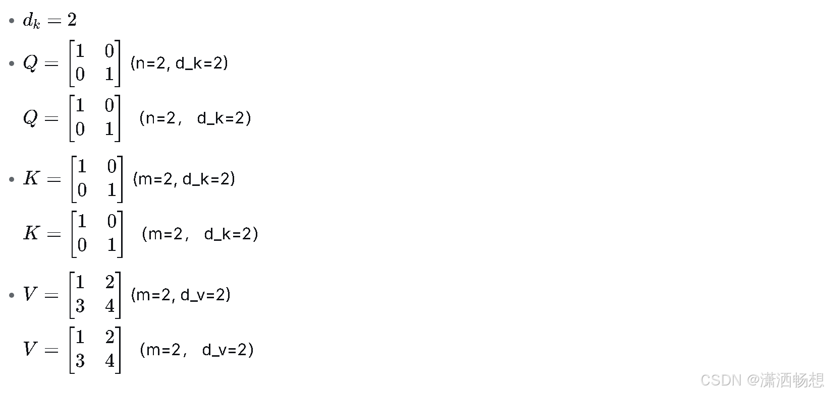
手动计算详细步骤:
1. 计算 :
QK^T = \begin{bmatrix} 1 & 0 \\ 0 & 1 \end{bmatrix} \times \begin{bmatrix} 1 & 0 \\ 0 & 1 \end{bmatrix} = \begin{bmatrix} 1\cdot1+0\cdot0 & 1\cdot0+0\cdot1 \\ 0\cdot1+1\cdot0 & 0\cdot0+1\cdot1 \end{bmatrix} = \begin{bmatrix} 1 & 0 \\ 0 & 1 \end{bmatrix}2. 缩放因子:
\sqrt{d_k} = \sqrt{2} \approx 1.414213563. 缩放得分:
S_{\text{scaled}} = \frac{QK^T}{\sqrt{d_k}} = \begin{bmatrix} 0.7071 & 0 \\ 0 & 0.7071 \end{bmatrix}4. Softmax计算(对每一行):
对于第一行 0.7071,00.7071,0:
-
exp(0.7071) ≈ 2.028 经验值(0.7071) ≈ 2.028
-
exp(0) = 1 exp(0) = 1
-
sum = 3.028 和 = 3.028
-
softmax = 2.028/3.028, 1/3.028 ≈ 0.67, 0.33
Softmax = 2.028/3.028, 1/3.028 ≈ 0.67, 0.33
同理第二行也得 0.33, 0.67(因对称)
5. 注意力权重矩阵 AA:
A \approx \begin{bmatrix} 0.67 & 0.33 \\ 0.33 & 0.67 \end{bmatrix}6. 输出 AV:
AV = \begin{bmatrix} 0.67\times1 + 0.33\times3 & 0.67\times2 + 0.33\times4 \\ 0.33\times1 + 0.67\times3 & 0.33\times2 + 0.67\times4 \end{bmatrix} = \begin{bmatrix} 1.66 & 2.66 \\ 2.34 & 3.34 \end{bmatrix}3.5 Step 4: 写代码
Python + NumPy实现 Python + NumPy 实现
import numpy as np

def scaled_dot_product_attention(Q, K, V):
    """
    缩放点积注意力
    Q: (n, d_k)
    K: (m, d_k)
    V: (m, d_v)
    返回: (n, d_v)
    """
    d_k = Q.shape[-1]
    # 1. 得分矩阵
    scores = np.matmul(Q, K.T)  # (n, m)
    # 2. 缩放
    scores = scores / np.sqrt(d_k)
    # 3. softmax每行(数值稳定版)
    exp_scores = np.exp(scores - np.max(scores, axis=1, keepdims=True))
    attention_weights = exp_scores / np.sum(exp_scores, axis=1, keepdims=True)
    # 4. 加权求和
    output = np.matmul(attention_weights, V)
    return output

# 测试
Q = np.array([[1, 0], [0, 1]])
K = np.array([[1, 0], [0, 1]])
V = np.array([[1, 2], [3, 4]])
print(scaled_dot_product_attention(Q, K, V))
Java实现(使用EJML库)
import org.ejml.simple.SimpleMatrix;

public class Attention {
    public static SimpleMatrix scaledDotProductAttention(
            SimpleMatrix Q, SimpleMatrix K, SimpleMatrix V) {
        int d_k = Q.numCols();
        // 1. 得分矩阵
        SimpleMatrix scores = Q.mult(K.transpose());
        // 2. 缩放
        scores = scores.divide(Math.sqrt(d_k));
        // 3. softmax每行
        SimpleMatrix expScores = scores.elementExp();
        SimpleMatrix rowSums = expScores.rowSums();
        SimpleMatrix attentionWeights = new SimpleMatrix(expScores);
        for (int i = 0; i < attentionWeights.numRows(); i++) {
            for (int j = 0; j < attentionWeights.numCols(); j++) {
                attentionWeights.set(i, j,
                    expScores.get(i, j) / rowSums.get(i, 0));
            }
        }
        // 4. 输出
        return attentionWeights.mult(V);
    }
}
Go实现(使用Gonum)
package main

import (
    "math"
    "gonum.org/v1/gonum/mat"
)

func softmaxRow(m *mat.Dense) *mat.Dense {
    r, c := m.Dims()
    result := mat.NewDense(r, c, nil)
    for i := 0; i < r; i++ {
        row := m.RowView(i)
        max := mat.Max(row)
        sum := 0.0
        for j := 0; j < c; j++ {
            val := math.Exp(m.At(i, j) - max)
            result.Set(i, j, val)
            sum += val
        }
        for j := 0; j < c; j++ {
            result.Set(i, j, result.At(i, j)/sum)
        }
    }
    return result
}

func scaledDotProductAttention(Q, K, V *mat.Dense) *mat.Dense {
    _, d_k := Q.Dims()
    var scores mat.Dense
    scores.Mul(Q, K.T())
    scores.Scale(1.0/math.Sqrt(float64(d_k)), &scores)
    attentionWeights := softmaxRow(&scores)
    var output mat.Dense
    output.Mul(attentionWeights, V)
    return &output
}
Rust实现(使用ndarray)
use ndarray::{Array2, Axis};
use ndarray_stats::QuantileExt;

fn softmax_row(mut scores: Array2<f64>) -> Array2<f64> {
    for mut row in scores.rows_mut() {
        let max = row.max().unwrap().clone();
        row.mapv_inplace(|x| (x - max).exp());
        let sum = row.sum();
        row.mapv_inplace(|x| x / sum);
    }
    scores
}

fn scaled_dot_product_attention(
    q: &Array2<f64>,
    k: &Array2<f64>,
    v: &Array2<f64>,
) -> Array2<f64> {
    let d_k = q.shape()[1] as f64;
    let scores = q.dot(&k.t()) / d_k.sqrt();
    let attention_weights = softmax_row(scores);
    attention_weights.dot(v)
}
C++实现(使用Eigen)
#include <Eigen/Dense>
#include <cmath>

Eigen::MatrixXd softmax_row(const Eigen::MatrixXd& scores) {
    Eigen::MatrixXd exp_scores =
        (scores.rowwise() - scores.colwise().maxCoeff()).array().exp();
    Eigen::VectorXd row_sums = exp_scores.rowwise().sum();
    return exp_scores.array().colwise() / row_sums.array();
}

Eigen::MatrixXd scaled_dot_product_attention(
    const Eigen::MatrixXd& Q,
    const Eigen::MatrixXd& K,
    const Eigen::MatrixXd& V)
{
    int d_k = Q.cols();
    Eigen::MatrixXd scores = Q * K.transpose() / std::sqrt(double(d_k));
    Eigen::MatrixXd attention_weights = softmax_row(scores);
    return attention_weights * V;
}
4. 实战二:拆解Batch Normalization公式
4.1 原始公式

LaTeX源码(可复制)
\hat{x}_i = \frac{x_i - \mu_{\mathcal{B}}}{\sqrt{\sigma_{\mathcal{B}}^2 + \epsilon}}, \quad y_i = \gamma \hat{x}_i + \beta4.2 四步拆解
| 步骤 | 内容 |
|---|---|
| 识符号 | xix i :输入;μBμ B:小批量均值;σB2σ B2:小批量方差;ϵϵ :极小常数(如1e-5)防止除零;γγ :可学习缩放参数;ββ xix i μBμ B σ 𝐵 2 S B 2ϵϵ γγ ββ:可学习平移参数 |
| 找结构 | 先标准化(减均值除以标准差)使分布变为N(0,1),再通过γ和β进行线性变换恢复表达能力 |
| 代数值 | 输入2, 4,均值=3,方差=1,ε=1e-5,γ=2,β=1 → 标准化得-1, 1 → 输出-1, 3 |
| 写代码 | 见下方多语言实现 |
4.3 代码实现
Python
import numpy as np

def batch_norm_1d(x, gamma, beta, eps=1e-5):
    mu = np.mean(x)
    var = np.var(x)
    x_hat = (x - mu) / np.sqrt(var + eps)
    return gamma * x_hat + beta
Java
public static double[] batchNorm(double[] x, double gamma, double beta, double eps) {
    double mu = Arrays.stream(x).average().orElse(0.0);
    double var = Arrays.stream(x).map(v -> Math.pow(v - mu, 2)).average().orElse(0.0);
    return Arrays.stream(x)
        .map(v -> gamma * (v - mu) / Math.sqrt(var + eps) + beta)
        .toArray();
}
JavaScript
const batchNorm = (x, gamma, beta, eps = 1e-5) => {
    const mu = x.reduce((a, b) => a + b) / x.length;
    const var_ = x.reduce((s, v) => s + (v - mu) ** 2, 0) / x.length;
    return x.map(v => gamma * (v - mu) / Math.sqrt(var_ + eps) + beta);
};
Go
func batchNorm(x []float64, gamma, beta, eps float64) []float64 {
    mu := mean(x)
    var_ := variance(x, mu)
    result := make([]float64, len(x))
    for i, v := range x {
        result[i] = gamma*(v-mu)/math.Sqrt(var_+eps) + beta
    }
    return result
}
Rust
fn batch_norm(x: &[f64], gamma: f64, beta: f64, eps: f64) -> Vec<f64> {
    let mu = x.iter().sum::<f64>() / x.len() as f64;
    let var = x.iter().map(|&v| (v - mu).powi(2)).sum::<f64>() / x.len() as f64;
    x.iter().map(|&v| gamma * (v - mu) / (var + eps).sqrt() + beta).collect()
}
C++
#include <vector>
#include <cmath>

std::vector<double> batchNorm(const std::vector<double>& x,
                               double gamma, double beta, double eps) {
    double mu = mean(x);
    double var = 0.0;
    for (double v : x) var += (v - mu) * (v - mu);
    var /= x.size();

    std::vector<double> result;
    for (double v : x) {
        result.push_back(gamma * (v - mu) / std::sqrt(var + eps) + beta);
    }
    return result;
}
5. 实战三:拆解交叉熵损失函数
5.1 原始公式

LaTeX源码(可复制)
\mathcal{L} = -\frac{1}{N} \sum_{i=1}^{N} \sum_{c=1}^{C} y_{i,c} \log(p_{i,c})5.2 四步拆解
| 步骤 | 内容 |
|---|---|
| 识符号 | LL:损失值;NN:样本数;CC:类别数;yi,cyi,c:第i个样本属于第c类的真实标签(one-hot);pi,cpi,c:模型预测概率 |
| 找结构 | 对每个样本的每个类别,计算真实标签与预测概率对数的乘积,求和,取平均,加负号 |
| 代数值 | 样本1:真实类别为2(one-hot 0,1,0),预测概率0.2,0.7,0.1 → 损失 = -log(0.7) ≈ 0.3567 |
| 写代码 | 见下方 |
5.3 代码实现
Python
def cross_entropy_loss(y_true, y_pred, eps=1e-12):
    """
    y_true: (N, C) one-hot 或 (N,) 类索引
    y_pred: (N, C) 预测概率
    """
    y_pred = np.clip(y_pred, eps, 1 - eps)  # 防止log(0)
    if y_true.ndim == 1:
        n = y_true.shape[0]
        c = y_pred.shape[1]
        y_true_onehot = np.zeros((n, c))
        y_true_onehot[np.arange(n), y_true] = 1
        y_true = y_true_onehot
    loss = -np.sum(y_true * np.log(y_pred)) / y_true.shape[0]
    return loss
Java
public static double crossEntropyLoss(int[] yTrue, double[][] yPred, double eps) {
    int n = yTrue.length;
    double loss = 0.0;
    for (int i = 0; i < n; i++) {
        loss -= Math.log(Math.max(yPred[i][yTrue[i]], eps));
    }
    return loss / n;
}
JavaScript
function crossEntropyLoss(yTrue, yPred, eps = 1e-12) {
    const n = yTrue.length;
    let loss = 0;
    for (let i = 0; i < n; i++) {
        loss -= Math.log(Math.max(yPred[i][yTrue[i]], eps));
    }
    return loss / n;
}
6. 更多公式阅读挑战
6.1 均方根误差RMSE

提示:四步拆解后,与MSE的区别仅在于多了一层开方,用于保持量纲一致。
6.2 余弦相似度

LaTeX源码
\text{similarity} = \cos(\theta) = \frac{\mathbf{A} \cdot \mathbf{B}}{\|\mathbf{A}\| \|\mathbf{B}\|}提示:点积除以模长乘积。注意分母为零的情况。
6.3 Sigmoid函数

提示 :常用于二分类输出,值域(0,1)。求导性质
6.4 Softmax函数

LaTeX源码
\text{softmax}(x_i) = \frac{e^{x_i}}{\sum_{j=1}^{K} e^{x_j}}提示:将K维向量映射为概率分布,注意数值稳定性(减去最大值)。
7. 本节小结:你的公式阅读工具箱
| 工具 | 内容 |
|---|---|
| 希腊字母速查表 | 16个高频字母的读音与代码映射 |
| 四步拆解法 | 识符号 → 找结构 → 代数值 → 写代码 |
| 实战案例 | Transformer注意力、BatchNorm、交叉熵损失 |
| 代码模板库 | Python/Java/JS/Go/Rust/C++六语言对照 |
| 扩展练习 | 4个额外公式供自主拆解 |
课后习题
基础题(必做)
题1(连线题):将下列希腊字母与其常见代码场景连线。
-
α ● 动量参数
-
β ● 均值
-
γ ● 学习率
-
λ ● 折扣因子
-
μ ● 正则化系数
-
σ ● 标准差
题2(拆解练习) :使用四步拆解法分析 Sigmoid函数,写出每一步的结果,并用Python实现。额外要求:实现其导数函数。
面试题(大厂高频)
题3(类似字节跳动):简述Transformer中为什么使用缩放点积注意力而不是普通点积注意力?如果 dkdk 很大,不缩放会有什么后果?(提示:softmax的梯度特性)
题4(类似阿里):Batch Normalization在训练和推理时的计算有何不同?请写出推理时的计算公式,并解释为什么可以这样简化。
扩展题(论文阅读)
题5 :阅读 Adam: A Method for Stochastic Optimization 论文中的参数更新公式:

LaTeX源码
m_t = \beta_1 m_{t-1} + (1-\beta_1) g_t, \quad v_t = \beta_2 v_{t-1} + (1-\beta_2) g_t^2

\hat{m}_t = \frac{m_t}{1-\beta_1^t}, \quad \hat{v}_t = \frac{v_t}{1-\beta_2^t}, \quad \theta_t = \theta_{t-1} - \alpha \frac{\hat{m}_t}{\sqrt{\hat{v}_t} + \epsilon}
用四步法写出拆解笔记,并尝试用伪代码描述完整更新流程。
题6(综合编码):请用你最擅长的语言,实现一个完整的Softmax函数,要求:
-
支持任意形状的二维张量(矩阵)
-
包含数值稳定处理(减去最大值)
-
附带测试用例验证输出每行和为1
附录:本节符号与公式LaTeX源码汇总
| 公式名称 | LaTeX源码 |
|---|---|
| Transformer注意力 | \text{Attention}(Q, K, V) = \text{softmax}\left( \frac{QK^T}{\sqrt{d_k}} \right) V \text{Attention}(Q, K, V) = \text{softmax}\left( \frac{QK^T}{\sqrt{d_k}} \right) V |
| BatchNorm 批次规范 | \hat{x}_i = \frac{x_i - \mu_{\mathcal{B}}}{\sqrt{\sigma_{\mathcal{B}}^2 + \epsilon}}, \quad y_i = \gamma \hat{x}_i + \beta \hat{x}i = \frac{x_i - \mu{\mathcal{B}}{\sqrt{\sigma_{\mathcal{B}}^2 + \epsilon}}, \quad y_i = \gamma \hat{x}_i + \beta |
| 交叉熵损失 | \mathcal{L} = -\frac{1}{N} \sum_{i=1}^{N} \sum_{c=1}^{C} y_{i,c} \log(p_{i,c}) \mathcal{L} = -\frac{1}{N} \sum_{i=1}^{N} \sum_{c=1}^{C} y_{i,c} \log(p_{i,c}) |
| RMSE | \text{RMSE} = \sqrt{ \frac{1}{n} \sum_{i=1}^{n} (y_i - \hat{y}_i)^2 } \text{RMSE} = \sqrt{ \frac{1}{n} \sum_{i=1}^{n} (y_i - \hat{y}_i)^2 } |
| 余弦相似度 | `\text{similarity} = \cos(\theta) = \frac{\mathbf{A} \cdot \mathbf{B}}{ |
| Sigmoid 乙状结肠 | \sigma(x) = \frac{1}{1 + e^{-x}} \sigma(x) = \frac{1}{1 + e^{-x}} |
| Softmax | \text{softmax}(x_i) = \frac{e^{x_i}}{\sum_{j=1}^{K} e^{x_j}} \text{softmax}(x_i) = \frac{e^{x_i}}{\sum_{j=1}^{K} e^{x_j}} |
本文配套代码已更新至GitHub仓库 self-learners-league/beauty-of-operators-and-formulas ,各语言实现见
volume1/chapter1/1.2_greek_alphabet/目录。习题答案将在上册完结后的《上册总结》中统一发布。
本文为《算符与公式之美·高级卷(上册)》第1章第2节内容,版权所有,未经授权禁止转载。