Day 15 编程实战：KMeans聚类与股票风格分类

Day 15 编程实战：KMeans聚类与股票风格分类

实战目标

1. 理解KMeans聚类算法的原理
2. 掌握肘部法则和轮廓系数选择K值
3. 理解初始化问题（KMeans++）
4. 对A股股票进行风格分类
5. 分析和解释聚类结果

1. 导入必要的库

import numpy as np
import pandas as pd
import matplotlib.pyplot as plt
import seaborn as sns
from sklearn.cluster import KMeans
from sklearn.preprocessing import StandardScaler, MinMaxScaler
from sklearn.decomposition import PCA
from sklearn.metrics import silhouette_score, silhouette_samples, calinski_harabasz_score
from scipy.spatial.distance import cdist
import warnings
warnings.filterwarnings('ignore')

sns.set_style("whitegrid")  # 预设样式
#启用LaTeX渲染（设为False避免LaTeX依赖）
plt.rcParams['text.usetex'] = False
# 设置中文显示
plt.rcParams['font.sans-serif'] = ['Microsoft YaHei', 'DejaVu Sans']
plt.rcParams['axes.unicode_minus'] = False
plt.rcParams['mathtext.fontset'] = 'dejavusans'  # 或 'stix'

2. 生成模拟股票数据

def generate_stock_data(n_stocks=300, seed=42):
    """
    生成模拟股票数据（沪深300风格）
    
    特征说明：
    - pe: 市盈率 (5-50，价值股低，成长股高)
    - pb: 市净率 (0.5-10)
    - roe: 净资产收益率 (-20% - 30%)
    - turnover: 换手率 (1%-20%)
    - growth: 营收增长率 (-10% - 50%)
    """
    np.random.seed(seed)
    
    n = n_stocks
    
    # 生成不同风格的股票
    # 价值股（约80只）
    n_value = 80
    value_pe = np.random.uniform(5, 15, n_value)
    value_pb = np.random.uniform(0.5, 1.5, n_value)
    value_roe = np.random.uniform(8, 20, n_value)
    value_turnover = np.random.uniform(1, 5, n_value)
    value_growth = np.random.uniform(0, 15, n_value)
    
    # 成长股（约80只）
    n_growth = 80
    growth_pe = np.random.uniform(25, 45, n_growth)
    growth_pb = np.random.uniform(3, 8, n_growth)
    growth_roe = np.random.uniform(10, 25, n_growth)
    growth_turnover = np.random.uniform(5, 15, n_growth)
    growth_growth = np.random.uniform(20, 45, n_growth)
    
    # 盈利股（高ROE，约70只）
    n_profitable = 70
    prof_pe = np.random.uniform(15, 25, n_profitable)
    prof_pb = np.random.uniform(1.5, 3, n_profitable)
    prof_roe = np.random.uniform(18, 30, n_profitable)
    prof_turnover = np.random.uniform(3, 8, n_profitable)
    prof_growth = np.random.uniform(8, 20, n_profitable)
    
    # 高换手股（热门股，约70只）
    n_hot = 70
    hot_pe = np.random.uniform(20, 50, n_hot)
    hot_pb = np.random.uniform(2, 10, n_hot)
    hot_roe = np.random.uniform(-5, 15, n_hot)
    hot_turnover = np.random.uniform(12, 20, n_hot)
    hot_growth = np.random.uniform(5, 30, n_hot)
    
    # 合并数据
    pe = np.concatenate([value_pe, growth_pe, prof_pe, hot_pe])
    pb = np.concatenate([value_pb, growth_pb, prof_pb, hot_pb])
    roe = np.concatenate([value_roe, growth_roe, prof_roe, hot_roe])
    turnover = np.concatenate([value_turnover, growth_turnover, prof_turnover, hot_turnover])
    growth = np.concatenate([value_growth, growth_growth, prof_growth, hot_growth])
    
    # 添加噪声
    pe += np.random.randn(n) * 2
    pb += np.random.randn(n) * 0.3
    roe += np.random.randn(n) * 2
    turnover += np.random.randn(n) * 1
    growth += np.random.randn(n) * 3
    
    # 创建DataFrame
    df = pd.DataFrame({
        'stock_id': [f'股票_{i+1:03d}' for i in range(n)],
        'pe': np.clip(pe, 0, 60),
        'pb': np.clip(pb, 0.3, 12),
        'roe': np.clip(roe, -30, 35),
        'turnover': np.clip(turnover, 0.5, 25),
        'growth': np.clip(growth, -10, 55)
    })
    
    # 添加真实标签（用于验证，实际聚类中不可知）
    true_labels = ['价值'] * n_value + ['成长'] * n_growth + ['盈利'] * n_profitable + ['热门'] * n_hot
    df['true_style'] = true_labels
    
    return df

# 生成数据
df_stock = generate_stock_data(n_stocks=300)
print(f"数据形状: {df_stock.shape}")
print(f"\n特征说明:")
print("  - pe: 市盈率（估值）")
print("  - pb: 市净率（估值）")
print("  - roe: 净资产收益率（盈利能力）")
print("  - turnover: 换手率（交易活跃度）")
print("  - growth: 营收增长率（成长性）")

print(f"\n数据统计:")
df_stock[['pe', 'pb', 'roe', 'turnover', 'growth']].describe()

# 显示前几行
df_stock.head()

数据形状: (300, 7)

特征说明:
  - pe: 市盈率（估值）
  - pb: 市净率（估值）
  - roe: 净资产收益率（盈利能力）
  - turnover: 换手率（交易活跃度）
  - growth: 营收增长率（成长性）

数据统计:

| | stock_id | pe | pb | roe | turnover | growth | true_style |
| 0 | 股票_001 | 3.746590 | 1.321567 | 15.693327 | 5.612732 | 5.150285 | 价值 |
| 1 | 股票_002 | 19.089028 | 0.756009 | 17.071925 | 4.678343 | 6.660928 | 价值 |
| 2 | 股票_003 | 9.540794 | 0.768191 | 15.753224 | 5.049922 | 5.335883 | 价值 |
| 3 | 股票_004 | 7.695787 | 0.308402 | 11.225365 | 2.377413 | 7.537074 | 价值 |

4	股票_005	8.605327	0.636825	8.591352	1.327189	12.435189	价值

3. 数据探索与可视化

# 查看真实风格分布
print("真实风格分布:")
print(df_stock['true_style'].value_counts())

# 可视化特征分布
fig, axes = plt.subplots(2, 3, figsize=(15, 10))

features = ['pe', 'pb', 'roe', 'turnover', 'growth']
colors = {'价值': 'blue', '成长': 'red', '盈利': 'green', '热门': 'orange'}

for idx, feature in enumerate(features):
    ax = axes[idx // 3, idx % 3]
    for style, color in colors.items():
        subset = df_stock[df_stock['true_style'] == style]
        ax.hist(subset[feature], bins=20, alpha=0.5, label=style, color=color)
    ax.set_xlabel(feature)
    ax.set_ylabel('频数')
    ax.set_title(f'{feature} 分布')
    ax.legend()
    ax.grid(True, alpha=0.3)

axes[1, 2].axis('off')
plt.suptitle('不同风格股票的特征分布', fontsize=14)
plt.tight_layout()
plt.show()

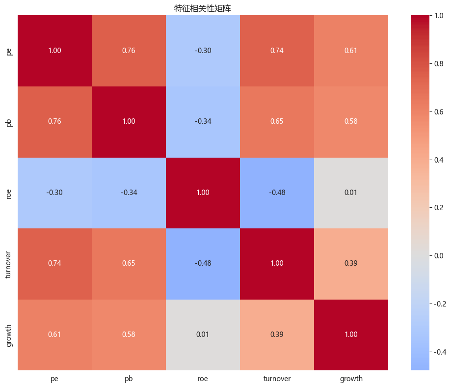
# 特征相关性热图
plt.figure(figsize=(10, 8))
corr_matrix = df_stock[['pe', 'pb', 'roe', 'turnover', 'growth']].corr()
sns.heatmap(corr_matrix, annot=True, fmt='.2f', cmap='coolwarm', center=0)
plt.title('特征相关性矩阵')
plt.tight_layout()
plt.show()

真实风格分布:
true_style
价值    80
成长    80
盈利    70
热门    70
Name: count, dtype: int64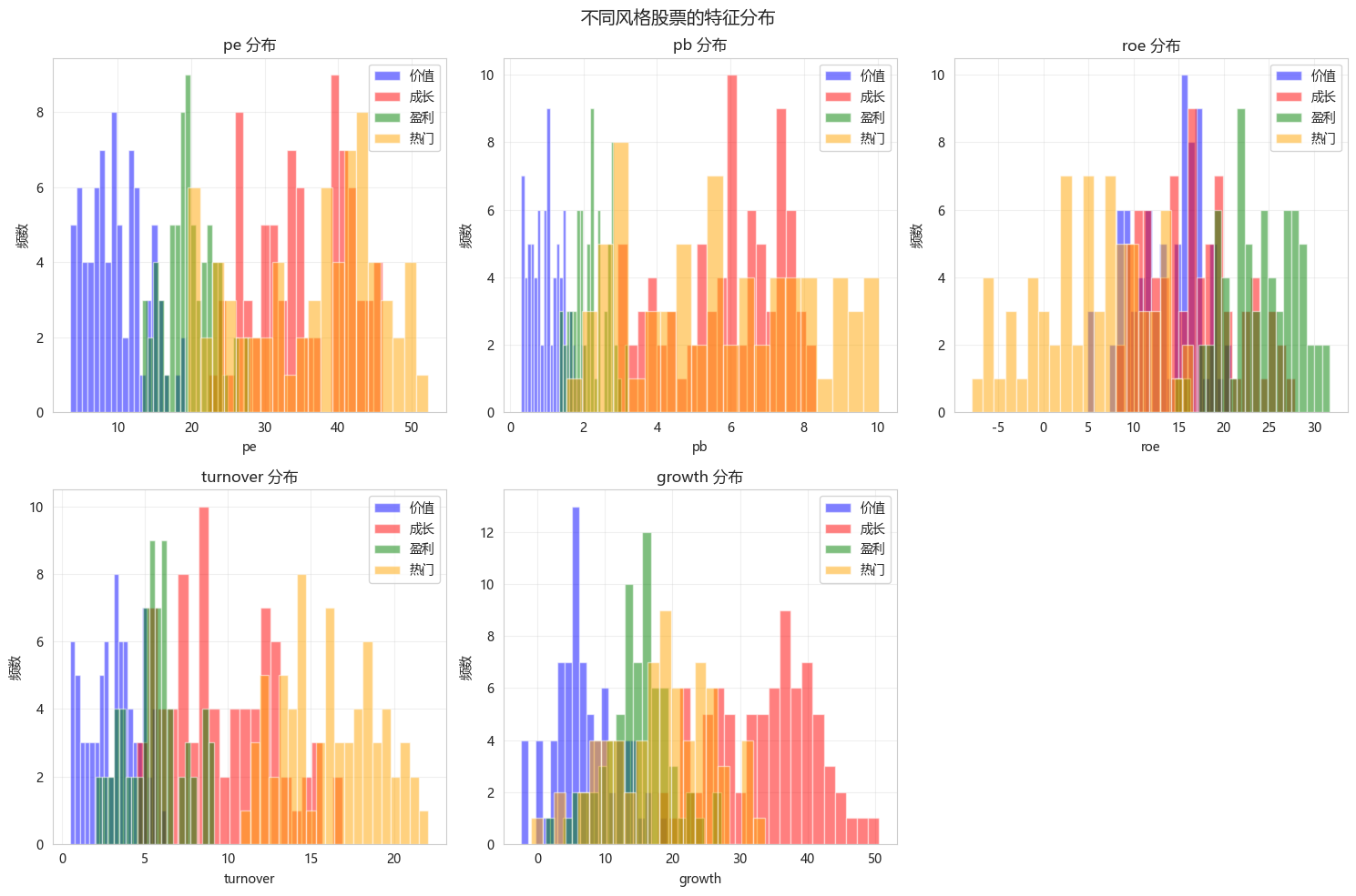

4. 数据预处理

# 提取特征
feature_cols = ['pe', 'pb', 'roe', 'turnover', 'growth']
X = df_stock[feature_cols].values

# 检查异常值
print("异常值检测（99%分位数）:")
for col in feature_cols:
    q99 = df_stock[col].quantile(0.99)
    q1 = df_stock[col].quantile(0.01)
    outliers_high = (df_stock[col] > q99).sum()
    outliers_low = (df_stock[col] < q1).sum()
    print(f"  {col}: 高异常值={outliers_high}, 低异常值={outliers_low}")

# 标准化（KMeans需要）
scaler = StandardScaler()
X_scaled = scaler.fit_transform(X)

# 创建标准化后的DataFrame便于分析
df_scaled = pd.DataFrame(X_scaled, columns=feature_cols)

print("\n标准化后特征统计:")
print(df_scaled.describe())

异常值检测（99%分位数）:
  pe: 高异常值=3, 低异常值=3
  pb: 高异常值=3, 低异常值=0
  roe: 高异常值=3, 低异常值=3
  turnover: 高异常值=3, 低异常值=3
  growth: 高异常值=3, 低异常值=3

标准化后特征统计:
                 pe            pb           roe      turnover      growth
count  3.000000e+02  3.000000e+02  3.000000e+02  3.000000e+02  300.000000
mean   2.131628e-16 -2.131628e-16  7.105427e-17  9.473903e-17    0.000000
std    1.001671e+00  1.001671e+00  1.001671e+00  1.001671e+00    1.001671
min   -1.686945e+00 -1.310600e+00 -2.818604e+00 -1.467075e+00   -1.795906
25%   -7.979561e-01 -8.367852e-01 -6.398222e-01 -7.918702e-01   -0.768477
50%   -1.536635e-01 -3.619340e-01  8.718569e-02 -3.479021e-01   -0.163231
75%    9.326276e-01  8.904222e-01  6.792770e-01  7.899057e-01    0.634017
max    2.132005e+00  2.447487e+00  2.098739e+00  2.507259e+00    2.746158

5. K值选择分析

5.1 肘部法则

def plot_elbow_method(X_scaled, max_k=15):
    """绘制肘部法则图"""
    inertias = []
    k_range = range(1, max_k + 1)
    
    for k in k_range:
        kmeans = KMeans(n_clusters=k, init='k-means++', random_state=42, n_init=10)
        kmeans.fit(X_scaled)
        inertias.append(kmeans.inertia_)
    
    plt.figure(figsize=(12, 5))
    
    plt.subplot(1, 2, 1)
    plt.plot(k_range, inertias, 'bo-', linewidth=2, markersize=8)
    plt.xlabel('K值')
    plt.ylabel('Inertia（簇内平方和）')
    plt.title('肘部法则选择K值')
    plt.grid(True, alpha=0.3)
    
    # 计算二阶导数找肘点
    plt.subplot(1, 2, 2)
    second_derivative = np.diff(np.diff(inertias))
    plt.plot(k_range[1:-1], second_derivative, 'ro-', linewidth=2, markersize=8)
    plt.axhline(y=0, color='k', linestyle='--', alpha=0.5)
    plt.xlabel('K值')
    plt.ylabel('Inertia二阶导数')
    plt.title('肘点检测（二阶导数）')
    plt.grid(True, alpha=0.3)
    
    elbow_idx = np.argmin(second_derivative) + 2
    plt.annotate(f'肘点 ≈ {elbow_idx}', xy=(elbow_idx, second_derivative[elbow_idx-2]), 
                 xytext=(elbow_idx+2, second_derivative[elbow_idx-2]+10),
                 arrowprops=dict(arrowstyle='->'))
    
    plt.tight_layout()
    plt.show()
    
    return inertias

inertias = plot_elbow_method(X_scaled)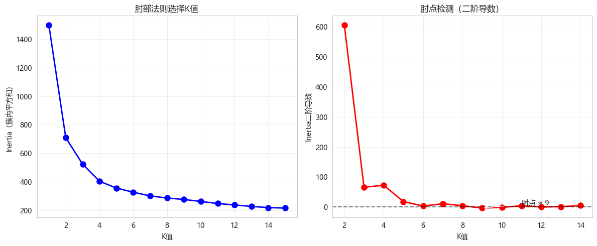

5.2 轮廓系数分析

def plot_silhouette_analysis(X_scaled, max_k=10):
    """绘制轮廓系数随K值变化"""
    silhouette_scores = []
    k_range = range(2, max_k + 1)
    
    for k in k_range:
        kmeans = KMeans(n_clusters=k, init='k-means++', random_state=42, n_init=10)
        labels = kmeans.fit_predict(X_scaled)
        score = silhouette_score(X_scaled, labels)
        silhouette_scores.append(score)
    
    plt.figure(figsize=(10, 6))
    plt.plot(k_range, silhouette_scores, 'go-', linewidth=2, markersize=8)
    plt.xlabel('K值')
    plt.ylabel('轮廓系数')
    plt.title('轮廓系数法选择K值（越大越好）')
    plt.axhline(y=0.5, color='r', linestyle='--', label='0.5阈值（良好分界）')
    plt.legend()
    plt.grid(True, alpha=0.3)
    plt.show()
    
    best_k = k_range[np.argmax(silhouette_scores)]
    print(f"最佳K值（轮廓系数）: {best_k}")
    print(f"最佳轮廓系数: {max(silhouette_scores):.4f}")
    
    return silhouette_scores

silhouette_scores = plot_silhouette_analysis(X_scaled)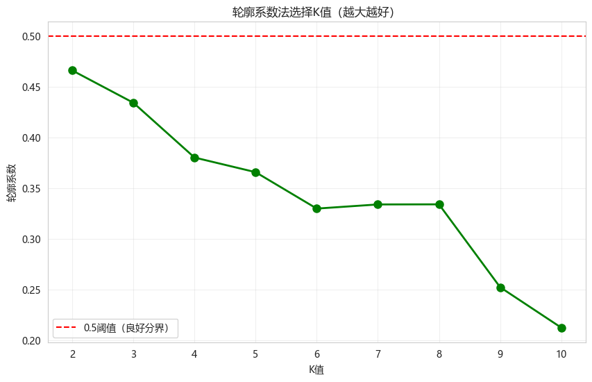

最佳K值（轮廓系数）: 2
最佳轮廓系数: 0.4660

5.3 轮廓系数可视化（K=4）

def plot_silhouette_for_k(X_scaled, k=4):
    """绘制特定K值的轮廓图"""
    kmeans = KMeans(n_clusters=k, init='k-means++', random_state=42, n_init=10)
    labels = kmeans.fit_predict(X_scaled)
    
    # 计算轮廓系数
    silhouette_vals = silhouette_samples(X_scaled, labels)
    silhouette_avg = silhouette_score(X_scaled, labels)
    
    print(f"K={k} 时的轮廓系数: {silhouette_avg:.4f}")
    
    # 绘制轮廓图
    fig, (ax1, ax2) = plt.subplots(1, 2, figsize=(14, 6))
    
    # 轮廓图
    y_lower = 10
    for i in range(k):
        cluster_vals = silhouette_vals[labels == i]
        cluster_vals.sort()
        y_upper = y_lower + len(cluster_vals)
        color = plt.cm.viridis(i / k)
        ax1.fill_betweenx(np.arange(y_lower, y_upper), 0, cluster_vals, 
                          facecolor=color, edgecolor=color, alpha=0.7)
        ax1.text(-0.05, y_lower + 0.5 * len(cluster_vals), str(i))
        y_lower = y_upper + 10
    
    ax1.axvline(x=silhouette_avg, color='red', linestyle='--', 
                label=f'平均轮廓系数={silhouette_avg:.3f}')
    ax1.set_xlabel('轮廓系数')
    ax1.set_ylabel('簇')
    ax1.set_title(f'轮廓图 (K={k})')
    ax1.legend()
    ax1.grid(True, alpha=0.3)
    
    # 簇大小分布
    cluster_sizes = pd.Series(labels).value_counts().sort_index()
    ax2.bar(cluster_sizes.index, cluster_sizes.values)
    ax2.set_xlabel('簇编号')
    ax2.set_ylabel('样本数')
    ax2.set_title('簇大小分布')
    ax2.grid(True, alpha=0.3)
    
    plt.tight_layout()
    plt.show()
    
    return labels

# 对K=4进行详细分析
labels_k4 = plot_silhouette_for_k(X_scaled, k=4)

K=4 时的轮廓系数: 0.3801

6. KMeans聚类模型训练

6.1 训练KMeans模型（K=4）

# 选择K=4（根据肘部法则和轮廓系数）
optimal_k = 4

kmeans = KMeans(n_clusters=optimal_k, init='k-means++', 
                n_init=20, max_iter=300, random_state=42)
labels = kmeans.fit_predict(X_scaled)

# 添加到DataFrame
df_stock['cluster'] = labels

# 评估指标
inertia = kmeans.inertia_
sil_score = silhouette_score(X_scaled, labels)
calinski_score = calinski_harabasz_score(X_scaled, labels)

print("="*60)
print("KMeans聚类结果")
print("="*60)
print(f"簇数 (K): {optimal_k}")
print(f"Inertia: {inertia:.4f}")
print(f"轮廓系数: {sil_score:.4f}")
print(f"Calinski-Harabasz指数: {calinski_score:.4f}")

# 簇分布
print(f"\n簇大小分布:")
for i in range(optimal_k):
    count = (labels == i).sum()
    print(f"  簇 {i}: {count} 只股票 ({count/len(labels):.1%})")

============================================================
KMeans聚类结果
============================================================
簇数 (K): 4
Inertia: 403.4727
轮廓系数: 0.3801
Calinski-Harabasz指数: 268.1487

簇大小分布:
  簇 0: 76 只股票 (25.3%)
  簇 1: 73 只股票 (24.3%)
  簇 2: 79 只股票 (26.3%)
  簇 3: 72 只股票 (24.0%)

6.2 初始化方法对比

def compare_initialization(X_scaled, k=4, n_runs=10):
    """对比KMeans++和随机初始化的效果"""
    
    kmeans_pp_inertias = []
    kmeans_random_inertias = []
    
    for seed in range(n_runs):
        # KMeans++
        kmeans_pp = KMeans(n_clusters=k, init='k-means++', random_state=seed, n_init=1)
        kmeans_pp.fit(X_scaled)
        kmeans_pp_inertias.append(kmeans_pp.inertia_)
        
        # 随机初始化
        kmeans_random = KMeans(n_clusters=k, init='random', random_state=seed, n_init=1)
        kmeans_random.fit(X_scaled)
        kmeans_random_inertias.append(kmeans_random.inertia_)
    
    plt.figure(figsize=(10, 6))
    plt.plot(range(n_runs), kmeans_pp_inertias, 'bo-', label='KMeans++', linewidth=2)
    plt.plot(range(n_runs), kmeans_random_inertias, 'rs-', label='随机初始化', linewidth=2)
    plt.xlabel('运行次数')
    plt.ylabel('Inertia')
    plt.title('初始化方法对比（越小越好）')
    plt.legend()
    plt.grid(True, alpha=0.3)
    plt.show()
    
    print(f"KMeans++ 平均 Inertia: {np.mean(kmeans_pp_inertias):.4f} ± {np.std(kmeans_pp_inertias):.4f}")
    print(f"随机初始化 平均 Inertia: {np.mean(kmeans_random_inertias):.4f} ± {np.std(kmeans_random_inertias):.4f}")
    print(f"KMeans++ 标准差更小，结果更稳定")

compare_initialization(X_scaled, k=optimal_k)

KMeans++ 平均 Inertia: 419.4458 ± 31.9251
随机初始化 平均 Inertia: 418.4479 ± 29.9295
KMeans++ 标准差更小，结果更稳定

7. 聚类结果分析与股票风格分类

7.1 各簇特征均值分析

# 计算每个簇的特征均值（原始尺度）
cluster_analysis = df_stock.groupby('cluster')[feature_cols].mean()
cluster_analysis_std = df_stock.groupby('cluster')[feature_cols].std()

print("="*60)
print("各簇特征均值（原始尺度）")
print("="*60)
print(cluster_analysis.round(2))

# 计算标准化后的特征均值（便于比较）
cluster_means_scaled = pd.DataFrame(X_scaled, columns=feature_cols)
cluster_means_scaled['cluster'] = labels
cluster_profile = cluster_means_scaled.groupby('cluster').mean()

print("\n各簇特征均值（标准化后，可跨特征比较）")
print(cluster_profile.round(3))

============================================================
各簇特征均值（原始尺度）
============================================================
            pe    pb    roe  turnover  growth
cluster                                      
0        35.08  5.90  16.50      9.57   33.94
1        19.76  2.23  23.89      5.60   15.07
2         9.83  1.00  13.46      3.16    6.82
3        36.58  5.82   5.37     16.02   18.70

各簇特征均值（标准化后，可跨特征比较）
            pe     pb    roe  turnover  growth
cluster                                       
0        0.785  0.851  0.207     0.203   1.319
1       -0.415 -0.567  1.123    -0.527  -0.298
2       -1.193 -1.042 -0.169    -0.977  -1.006
3        0.902  0.820 -1.172     1.392   0.013

7.2 风格标签分配

def assign_style_labels(cluster_profile):
    """根据簇特征均值分配风格标签"""
    style_labels = {}
    
    for cluster in cluster_profile.index:
        profile = cluster_profile.loc[cluster]
        
        # 价值股：低PE、低PB
        if profile['pe'] < -0.2 and profile['pb'] < -0.2:
            style_labels[cluster] = '价值股'
        # 成长股：高PE、高增长
        elif profile['pe'] > 0.3 and profile['growth'] > 0.3:
            style_labels[cluster] = '成长股'
        # 盈利股：高ROE
        elif profile['roe'] > 0.5:
            style_labels[cluster] = '盈利股'
        # 低估值股：低PE、低PB
        elif profile['pe'] < 0 and profile['pb'] < 0:
            style_labels[cluster] = '低估值股'
        # 高换手股：高换手率
        elif profile['turnover'] > 0.5:
            style_labels[cluster] = '活跃股'
        else:
            style_labels[cluster] = f'混合{cluster}'
    
    return style_labels

style_labels = assign_style_labels(cluster_profile)
df_stock['cluster_style'] = df_stock['cluster'].map(style_labels)

print("簇风格标签分配:")
for cluster, label in style_labels.items():
    print(f"  簇 {cluster}: {label}")
    
    # 显示该簇的特征均值
    means = cluster_profile.loc[cluster]
    print(f"     PE: {means['pe']:.2f}, PB: {means['pb']:.2f}, ROE: {means['roe']:.2f}, "
          f"换手率: {means['turnover']:.2f}, 增长: {means['growth']:.2f}")

簇风格标签分配:
  簇 0: 成长股
     PE: 0.78, PB: 0.85, ROE: 0.21, 换手率: 0.20, 增长: 1.32
  簇 1: 价值股
     PE: -0.42, PB: -0.57, ROE: 1.12, 换手率: -0.53, 增长: -0.30
  簇 2: 价值股
     PE: -1.19, PB: -1.04, ROE: -0.17, 换手率: -0.98, 增长: -1.01
  簇 3: 活跃股
     PE: 0.90, PB: 0.82, ROE: -1.17, 换手率: 1.39, 增长: 0.01

7.3 聚类结果可视化

# PCA降维可视化
pca = PCA(n_components=2)
X_pca = pca.fit_transform(X_scaled)

plt.figure(figsize=(12, 5))

plt.subplot(1, 2, 1)
scatter = plt.scatter(X_pca[:, 0], X_pca[:, 1], c=labels, cmap='viridis', s=50, alpha=0.7)
plt.colorbar(scatter, label='簇')
plt.xlabel('PC1')
plt.ylabel('PC2')
plt.title('KMeans聚类结果（PCA降维）')
plt.grid(True, alpha=0.3)

# 按风格着色
plt.subplot(1, 2, 2)
style_colors = {'价值股': 'blue', '成长股': 'red', '盈利股': 'green', '活跃股': 'orange', '混合股': 'purple'}
for style, color in style_colors.items():
    mask = df_stock['cluster_style'] == style
    if mask.sum() > 0:
        plt.scatter(X_pca[mask, 0], X_pca[mask, 1], c=color, label=style, s=50, alpha=0.7)
plt.xlabel('PC1')
plt.ylabel('PC2')
plt.title('聚类风格标签（PCA降维）')
plt.legend()
plt.grid(True, alpha=0.3)

plt.tight_layout()
plt.show()

# 解释PCA方差
print(f"PCA解释方差比例: PC1={pca.explained_variance_ratio_[0]:.2%}, PC2={pca.explained_variance_ratio_[1]:.2%}")

PCA解释方差比例: PC1=60.90%, PC2=21.28%

7.4 各簇特征雷达图

def plot_cluster_radar(cluster_profile, style_labels):
    """绘制各簇的特征雷达图"""
    from math import pi
    
    features = cluster_profile.columns.tolist()
    n_features = len(features)
    
    # 添加闭包
    angles = [n / n_features * 2 * pi for n in range(n_features)]
    angles += angles[:1]
    
    fig, ax = plt.subplots(figsize=(10, 10), subplot_kw={'projection': 'polar'})
    
    colors = ['blue', 'red', 'green', 'orange', 'purple']
    
    for i, (cluster, row) in enumerate(cluster_profile.iterrows()):
        values = row.values.tolist()
        values += values[:1]
        ax.plot(angles, values, 'o-', linewidth=2, label=style_labels[cluster], color=colors[i % len(colors)])
        ax.fill(angles, values, alpha=0.1, color=colors[i % len(colors)])
    
    ax.set_xticks(angles[:-1])
    ax.set_xticklabels(features)
    ax.set_ylim(-1.5, 2)
    ax.set_title('各簇特征雷达图（标准化后）', size=15)
    ax.legend(loc='upper right', bbox_to_anchor=(1.3, 1.0))
    plt.tight_layout()
    plt.show()

plot_cluster_radar(cluster_profile, style_labels)

7.5 簇特征箱线图

fig, axes = plt.subplots(2, 3, figsize=(15, 10))
axes = axes.ravel()

for idx, feature in enumerate(feature_cols):
    ax = axes[idx]
    data = [df_stock[df_stock['cluster'] == i][feature] for i in range(optimal_k)]
    bp = ax.boxplot(data, labels=[f'簇{i}' for i in range(optimal_k)], patch_artist=True)
    for patch, color in zip(bp['boxes'], ['blue', 'red', 'green', 'orange']):
        patch.set_facecolor(color)
    ax.set_ylabel(feature)
    ax.set_title(f'{feature} 分布')
    ax.grid(True, alpha=0.3)

axes[5].axis('off')
plt.suptitle('各簇特征分布箱线图', fontsize=14)
plt.tight_layout()
plt.show()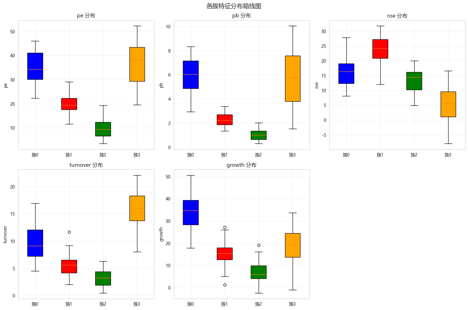

8. 聚类验证：与真实风格对比

# 创建混淆矩阵（聚类 vs 真实风格）
confusion = pd.crosstab(df_stock['true_style'], df_stock['cluster_style'])
print("="*60)
print("聚类结果 vs 真实风格对比")
print("="*60)
print(confusion)

# 计算调整兰德指数（ARI）
from sklearn.metrics import adjusted_rand_score, normalized_mutual_info_score

# 将风格标签转换为数值
style_to_num = {style: i for i, style in enumerate(df_stock['true_style'].unique())}
true_numeric = df_stock['true_style'].map(style_to_num).values

ari = adjusted_rand_score(true_numeric, labels)
nmi = normalized_mutual_info_score(true_numeric, labels)

print(f"\n调整兰德指数 (ARI): {ari:.4f}")
print(f"归一化互信息 (NMI): {nmi:.4f}")
print("ARI和NMI范围[-1,1]/[0,1]，越大表示聚类与真实标签越一致")

============================================================
聚类结果 vs 真实风格对比
============================================================
cluster_style  价值股  成长股  活跃股
true_style                  
价值              80    0    0
成长               1   76    3
热门               1    0   69
盈利              70    0    0

调整兰德指数 (ARI): 0.9303
归一化互信息 (NMI): 0.9092
ARI和NMI范围[-1,1]/[0,1]，越大表示聚类与真实标签越一致

9. 聚类结果解读与投资启示

print("="*70)
print("股票风格分类结果解读")
print("="*70)

for cluster in range(optimal_k):
    style = style_labels[cluster]
    stocks_in_cluster = df_stock[df_stock['cluster'] == cluster]
    n_stocks = len(stocks_in_cluster)
    
    # 特征均值
    means = cluster_analysis.loc[cluster]
    
    print(f"\n┌─────────────────────────────────────────────────────────────────────┐")
    print(f"│ 簇 {cluster}: {style} ({n_stocks}只股票)                              ")
    print(f"├─────────────────────────────────────────────────────────────────────┤")
    print(f"│ 特征画像:                                                          ")
    print(f"│   - 市盈率(PE): {means['pe']:.1f} (行业均值约20)                      ")
    print(f"│   - 市净率(PB): {means['pb']:.2f} (行业均值约2)                       ")
    print(f"│   - ROE: {means['roe']:.1f}% (行业均值约10%)                         ")
    print(f"│   - 换手率: {means['turnover']:.1f}% (行业均值约8%)                    ")
    print(f"│   - 增长率: {means['growth']:.1f}% (行业均值约15%)                     ")
    print(f"├─────────────────────────────────────────────────────────────────────┤")
    
    # 投资建议
    if '价值' in style:
        print("│ 投资建议: 适合长期价值投资，关注估值修复机会                       ")
        print("│ 特征: 低估值、稳定盈利、换手率低                                  ")
    elif '成长' in style:
        print("│ 投资建议: 适合成长型投资，关注业绩增速                           ")
        print("│ 特征: 高估值、高增长、ROE良好                                    ")
    elif '盈利' in style:
        print("│ 投资建议: 适合获取稳定收益，关注ROE持续性                         ")
        print("│ 特征: 高ROE、中等估值、盈利能力强                                ")
    elif '活跃' in style:
        print("│ 投资建议: 适合短线交易，关注市场情绪和流动性                       ")
        print("│ 特征: 高换手率、估值波动大                                       ")
    else:
        print("│ 投资建议: 需要进一步分析基本面                                    ")
        print("│ 特征: 各项指标较为均衡                                           ")
    
    print("└─────────────────────────────────────────────────────────────────────┘")

======================================================================
股票风格分类结果解读
======================================================================

┌─────────────────────────────────────────────────────────────────────┐
│ 簇 0: 成长股 (76只股票)                              
├─────────────────────────────────────────────────────────────────────┤
│ 特征画像:                                                          
│   - 市盈率(PE): 35.1 (行业均值约20)                      
│   - 市净率(PB): 5.90 (行业均值约2)                       
│   - ROE: 16.5% (行业均值约10%)                         
│   - 换手率: 9.6% (行业均值约8%)                    
│   - 增长率: 33.9% (行业均值约15%)                     
├─────────────────────────────────────────────────────────────────────┤
│ 投资建议: 适合成长型投资，关注业绩增速                           
│ 特征: 高估值、高增长、ROE良好                                    
└─────────────────────────────────────────────────────────────────────┘

┌─────────────────────────────────────────────────────────────────────┐
│ 簇 1: 价值股 (73只股票)                              
├─────────────────────────────────────────────────────────────────────┤
│ 特征画像:                                                          
│   - 市盈率(PE): 19.8 (行业均值约20)                      
│   - 市净率(PB): 2.23 (行业均值约2)                       
│   - ROE: 23.9% (行业均值约10%)                         
│   - 换手率: 5.6% (行业均值约8%)                    
│   - 增长率: 15.1% (行业均值约15%)                     
├─────────────────────────────────────────────────────────────────────┤
│ 投资建议: 适合长期价值投资，关注估值修复机会                       
│ 特征: 低估值、稳定盈利、换手率低                                  
└─────────────────────────────────────────────────────────────────────┘

┌─────────────────────────────────────────────────────────────────────┐
│ 簇 2: 价值股 (79只股票)                              
├─────────────────────────────────────────────────────────────────────┤
│ 特征画像:                                                          
│   - 市盈率(PE): 9.8 (行业均值约20)                      
│   - 市净率(PB): 1.00 (行业均值约2)                       
│   - ROE: 13.5% (行业均值约10%)                         
│   - 换手率: 3.2% (行业均值约8%)                    
│   - 增长率: 6.8% (行业均值约15%)                     
├─────────────────────────────────────────────────────────────────────┤
│ 投资建议: 适合长期价值投资，关注估值修复机会                       
│ 特征: 低估值、稳定盈利、换手率低                                  
└─────────────────────────────────────────────────────────────────────┘

┌─────────────────────────────────────────────────────────────────────┐
│ 簇 3: 活跃股 (72只股票)                              
├─────────────────────────────────────────────────────────────────────┤
│ 特征画像:                                                          
│   - 市盈率(PE): 36.6 (行业均值约20)                      
│   - 市净率(PB): 5.82 (行业均值约2)                       
│   - ROE: 5.4% (行业均值约10%)                         
│   - 换手率: 16.0% (行业均值约8%)                    
│   - 增长率: 18.7% (行业均值约15%)                     
├─────────────────────────────────────────────────────────────────────┤
│ 投资建议: 适合短线交易，关注市场情绪和流动性                       
│ 特征: 高换手率、估值波动大                                       
└─────────────────────────────────────────────────────────────────────┘

10. 不同K值的对比试验

def compare_different_k(X_scaled, k_values=[3, 4, 5, 6]):
    """对比不同K值的聚类效果"""
    
    fig, axes = plt.subplots(2, 2, figsize=(14, 12))
    axes = axes.ravel()
    
    pca = PCA(n_components=2)
    X_pca = pca.fit_transform(X_scaled)
    
    results = []
    
    for idx, k in enumerate(k_values):
        kmeans = KMeans(n_clusters=k, init='k-means++', random_state=42, n_init=10)
        labels = kmeans.fit_predict(X_scaled)
        
        sil_score = silhouette_score(X_scaled, labels)
        calinski = calinski_harabasz_score(X_scaled, labels)
        
        results.append({
            'K': k,
            '轮廓系数': sil_score,
            'Calinski-Harabasz': calinski,
            'Inertia': kmeans.inertia_
        })
        
        axes[idx].scatter(X_pca[:, 0], X_pca[:, 1], c=labels, cmap='viridis', s=30, alpha=0.7)
        axes[idx].set_title(f'K={k} (轮廓系数={sil_score:.3f})')
        axes[idx].set_xlabel('PC1')
        axes[idx].set_ylabel('PC2')
        axes[idx].grid(True, alpha=0.3)
    
    plt.suptitle('不同K值的聚类效果对比', fontsize=14)
    plt.tight_layout()
    plt.show()
    
    results_df = pd.DataFrame(results)
    print("\n不同K值评估指标对比:")
    print(results_df.to_string(index=False))
    
    return results_df

compare_different_k(X_scaled, k_values=[3, 4, 5, 6])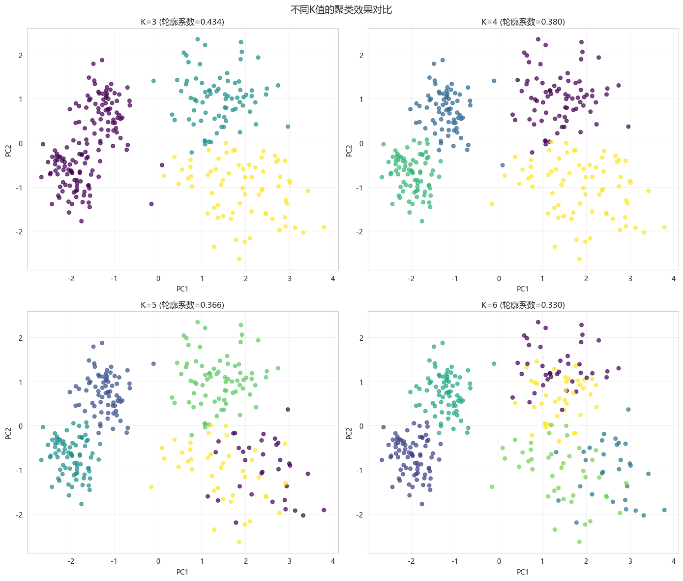

​

不同K值评估指标对比:
 K     轮廓系数  Calinski-Harabasz    Inertia
 3 0.434071         276.992200 523.511359
 4 0.380052         268.148729 403.472705
 5 0.365610         237.002966 355.990166
 6 0.329705         211.206760 326.658488

| | K | 轮廓系数 | Calinski-Harabasz | Inertia |
| 0 | 3 | 0.434071 | 276.992200 | 523.511359 |
| 1 | 4 | 0.380052 | 268.148729 | 403.472705 |
| 2 | 5 | 0.365610 | 237.002966 | 355.990166 |

3	6	0.329705	211.206760	326.658488

11. 今日总结

---

1. KMeans聚类核心概念 ：
   • 无监督学习，基于距离的聚类算法
   • 目标：最小化簇内平方和（Inertia）
   • 步骤：分配 → 更新 → 重复

---

2. K值选择方法 ：
   • 肘部法则：Inertia下降拐点
   • 轮廓系数：聚合/分离度，取值范围[-1,1]
   • 推荐综合使用多种方法

---

3. 初始化问题 ：
   • KMeans++：智能初始化，提高收敛质量
   • 多次运行取最优

---

4. 数据预处理 ：
   • 必须标准化（StandardScaler）
   • 处理异常值

---

5. 量化应用 ：
   • 股票风格分类（价值/成长/盈利/活跃）
   • 构建风格轮动策略
   • 风险分散化配置

---

6. 聚类结果解释 ：
   • 分析各簇特征均值
   • 可视化辅助理解
   • 结合业务知识命名

---

7. 扩展作业 ：
   • 作业1：尝试不同的聚类算法（层次聚类、DBSCAN），对比结果
   • 作业2：使用真实A股数据（通过akshare获取）进行聚类分析
   • 作业3：构建简单的风格轮动策略：根据市场环境选择不同风格的股票
   • 作业4：使用Gap统计量选择K值（高级）

---

8. 量化思考 ：
   • 聚类可以帮助发现股票的内在分组结构
   • 可以用于构建风格分散的投资组合
   • 定期重新聚类以适应市场风格变化
   • 结合基本面分析验证聚类结果

---

9. 聚类评估指标速查表：

   指标名称	范围	期望值	说明
   Inertia	[0, ∞)	越小越好	簇内平方和，越小越紧凑
   轮廓系数(Silhouette)	[-1, 1]	越接近1越好	综合评估聚合和分离
   Calinski-Harabasz	[0, ∞)	越大越好	簇间方差/簇内方差比
   Davies-Bouldin	[0, ∞)	越小越好	簇间相似度/簇内相似度比